Binod Kafle  ,
Ville Kankare,
Harri Kaartinen,
Kari Väätäinen,
Heikki Hyyti,
Tamas Faitli,
Juha Hyyppä,
Antero Kukko,
Kalle Kärhä
,
Ville Kankare,
Harri Kaartinen,
Kari Väätäinen,
Heikki Hyyti,
Tamas Faitli,
Juha Hyyppä,
Antero Kukko,
Kalle Kärhä
Assessing the consistency of low vegetation characteristics estimated using harvester, handheld, and drone light detection and ranging (LiDAR) systems
Kafle B., Kankare V., Kaartinen H., Väätäinen K., Hyyti H., Faitli T., Hyyppä J., Kukko A., Kärhä K. (2025). Assessing the consistency of low vegetation characteristics estimated using harvester, handheld, and drone light detection and ranging (LiDAR) systems. Silva Fennica vol. 59 no. 2 article id 25013. https://doi.org/10.14214/sf.25013
Highlights
- Harvester-mounted LiDAR consistently estimated low vegetation height and volume comparable to handheld and drone LiDAR
- Enhancing LiDAR range could improve harvester LiDAR efficiency, reducing processing time and increasing accuracy beyond 20 m.
Abstract
Evaluating the potential of a harvester-mounted LiDAR system in monitoring biodiversity indicators such as low vegetation during forest harvesting could enhance sustainable forest management and habitat conservation including dense forest areas for game. However, there is a lack of understanding on the capabilities and limitations of these systems to detect low vegetation characteristics. To address this knowledge gap, this study investigated the performance of a harvester-mounted LiDAR system for measuring low vegetation (height <5 m) attributes in a boreal forest in Finland, by comparing it with handheld mobile laser scanning (HMLS) and drone laser scanning (DLS) systems. LiDAR point cloud data was collected in September 2023 to quantify the low vegetation height (maximum, mean, and percentiles), volume (voxel-based and mean height-based) and cover (grid method). Depending on the system, LiDAR point cloud data was collected either before (HMLS and DLS), during (harvester LiDAR) or after (HMLS and DLS) harvesting operations. A total of 46 fixed-sized (5 m × 5 m) grid cells were studied and analyzed. Results showed harvester-mounted LiDAR provided consistent estimates with HMLS and DLS for maximum height, 99th height percentile, and volume across various grids (5 cm, 10 cm, 20 cm) and voxel (20 cm) sizes. High correlation was observed between the systems used for these attributes. This study demonstrated that harvester-mounted LiDAR is comparable to HMLS and DLS for assessing low vegetation height and volume. The findings could assist forest harvester operators in identifying potential low vegetation and dense areas for conservation and game management.
Keywords
biodiversity;
harvester;
wood harvesting;
dense area for games;
drone laser scanning (DLS);
handheld mobile laser scanning (HMLS);
point cloud
-
Kafle,
School of Forest Sciences, University of Eastern Finland (UEF), Yliopistokatu 7, FI-80101 Joensuu, Finland
 https://orcid.org/0000-0003-0744-3480
E-mail
binod.kafle@uef.fi
https://orcid.org/0000-0003-0744-3480
E-mail
binod.kafle@uef.fi
-
Kankare,
Department of Geography and Geology, University of Turku, FI-20014 Turun yliopisto, Finland
https://orcid.org/0000-0001-6038-1579
E-mail
viveka@utu.fi
-
Kaartinen,
Department of Remote Sensing and Photogrammetry, Finnish Geospatial Research Institute (FGI), Opastinsilta 12 C, FI-00520 Helsinki, Finland
https://orcid.org/0000-0002-4796-3942
E-mail
harri.kaartinen@nls.fi
-
Väätäinen,
Natural Resources Institute Finland (Luke), Yliopistokatu 6 B, FI-80100 Joensuu, Finland
https://orcid.org/0000-0002-6886-0432
E-mail
kari.vaatainen@luke.fi
-
Hyyti,
Department of Remote Sensing and Photogrammetry, Finnish Geospatial Research Institute (FGI), Opastinsilta 12 C, FI-00520 Helsinki, Finland
https://orcid.org/0000-0003-4664-6221
E-mail
heikki.hyyti@nls.fi
-
Faitli,
Department of Remote Sensing and Photogrammetry, Finnish Geospatial Research Institute (FGI), Opastinsilta 12 C, FI-00520 Helsinki, Finland
https://orcid.org/0000-0001-5334-5537
E-mail
tamas.faitli@nls.fi
- Hyyppä, Department of Remote Sensing and Photogrammetry, Finnish Geospatial Research Institute (FGI), Opastinsilta 12 C, FI-00520 Helsinki, Finland E-mail juha.coelasr@gmail.com
-
Kukko,
Department of Remote Sensing and Photogrammetry, Finnish Geospatial Research Institute (FGI), Opastinsilta 12 C, FI-00520 Helsinki, Finland
https://orcid.org/0000-0002-3841-6533
E-mail
antero.kukko@nls.fi
- Kärhä, School of Forest Sciences, University of Eastern Finland (UEF), Yliopistokatu 7, FI-80101 Joensuu, Finland E-mail kalle.karha@uef.fi
Received 27 April 2025 Accepted 12 August 2025 Published 21 August 2025
Views 49301
Available at https://doi.org/10.14214/sf.25013 | Download PDF

Supplementary Files
1 Introduction
A forest stand includes different stratum of vegetation, broadly categorized into low, medium, and high vegetation (Szostak and Pająk 2023). Low vegetation includes grasses, herbs, shrubs, and small trees (Frankenstein and Koenig 2004; Fu 2019). However, the definition of low vegetation varies in research, for example, up to 5 meters (m) (Fu 2019), 7 m (Szostak and Pająk 2023), and 8 m (Huo et al. 2022) from ground level. The terms of undergrowth, understorey, and understory (Kärhä 2006; Kärhä and Bergström 2020; Song et al. 2021; Adhikari et al. 2023; Ferrara et al. 2023; Penman et al. 2023; Yang et al. 2023) are also commonly used to describe the low vegetation between the forest floor and the dominant canopy layer. Low vegetation is essential for forest ecosystems contributing to biodiversity conservation and forest regeneration (George and Bazzaz 2014). Low vegetation participates in carbon, nutrient, and water cycling (Muller 2014; Elliott et al. 2015; Thrippleton et al. 2018; Landuyt et al. 2019; Balandier et al. 2022). Additionally, it provides food, shelter, and habitat for soil arthropods and large herbivores (Huffman et al. 2009; Boch et al. 2013).
To comprehensively quantify the structural characteristics such as vegetation density, cover, height, and volume of the low vegetation within a forest is challenging, time-consuming, and thus costly task to conduct with conventional field surveys (Tuanmu et al. 2010; Eskelson et al. 2020; Adhikari et al. 2023). These structural attributes are essential for estimating low vegetation biomass (Cooper et al. 2017; Sumnall et al. 2017; Adhikari et al. 2023), a fundamental indicator of forest ecosystem, forest productivity and carbon storage (Ma et al. 2024). Remote sensing technologies such as satellite imaging sensors offer a promising alternative for large-scale data collection with high temporal resolution but detecting the low vegetation characteristics is hindered by the dominant canopy layer interference and complex interactions affecting sensor signals (Eriksson et al. 2006; Tuanmu et al. 2010).
Active sensor technologies with light detection and ranging (LiDAR) technology have shown strong potential for accurately capturing the three-dimensional structure of low vegetation. Different LiDAR acquisition systems such as airborne laser scanning (ALS) (Sumnall et al. 2017; Campbell et al. 2018; Venier et al. 2019), terrestrial laser scanning (TLS) (Adhikari et al. 2023; Penman et al. 2023; Tienaho et al. 2024), integration of TLS with ALS (Ferrara et al. 2023), and mobile laser scanning (MLS) (Lin et al. 2014) have demonstrated the capability to quantify understory vegetation structure. Point cloud data, derived from these systems enable the extraction of key structural metrics, including height, volume, and cover. By capturing the three-dimensional (3D) distribution of vegetation, LiDAR data support the calculation of height metrics (e.g., maximum height, mean height, and height percentiles), voxel-based and area-weighted estimates of volume occupancy, and horizontal projections used to derive vegetation cover. Notably, Adhikari et al. (2023) reported a strong predictability (R2adj = 0.80) between LiDAR-derived volume occupancy and field-measured biomass of low vegetation, indicating that LiDAR point clouds are a reliable estimator of low vegetation volume.
While ALS is widely used for large-area data acquisition, MLS can serve as a complementary or alternative approach when high-resolution data over smaller areas are needed. MLS is particularly suitable for applications requiring very high point densities (e.g., 7000 points m⁻2; Nardinocchi and Esposito 2024). MLS is based on mobile platforms where LiDAR sensors and positioning systems, such as Global Navigation Satellite Systems (GNSSs) and Inertial Measurement Units (IMUs), are implemented to capture 3D point cloud data over forested areas (Kukko et al. 2017). MLS technology can also utilize automatic co-registration methods such as simultaneous localization and mapping (SLAM) to align point clouds without relying solely on GNSS system to provide sufficient position accuracy (Donager et al. 2021). However, MLS also has some limitations, such as lower point density and precision compared to TLS. For example, in diameter at breast height (DBH) measurement, MLS has a standard deviation of 3.7 cm, whereas TLS achieves 1.1 cm (Bienert et al. 2018). TLS typically provides a much higher point density, with values around 37 000 points m⁻2 (Torralba et al. 2022), which enhances the level of detail in measurements (Hyyppä et al. 2020; Stovall et al. 2023). MLS may struggle with occlusion issues in dense forest stands, potentially leading to incomplete data capture (shadowing effect) for upper canopy structures. Additionally, MLS systems may face challenges in maintaining consistent data quality across varying forest conditions and may require sophisticated algorithms for accurate tree detection and measurement (Hunčaga et al. 2020). Despite these limitations, ongoing advancements in MLS technology continue to improve data quality and processing methodologies, making it an increasingly valuable tool for forestry applications that require a balance between coverage area and data precision (Hyyppä et al. 2020; Faitli et al. 2024; Muhojoki et al. 2024).
Application of MLS in different mobile platforms such as vehicle-mounted (Bienert et al. 2018), backpack-mounted (Hyyppä et al. 2020; Hartley et al. 2022), handheld (Hyyppä et al. 2020; Jones et al. 2022), unmanned aerial vehicle (UAV) for under-canopy and above-canopy (Jaakkola et al. 2010; Torresan et al. 2017; Hyyppä et al. 2020) have been utilized in previous research. Sagar et al. (2024) demonstrated that a LiDAR system with an MLS sensor, mounted on a Cut-to-Length (CTL) harvester, achieved 100% accuracy in detecting tree stems. They also reported a Root Mean Square Error (RMSE) of 0.77% in detecting stem defects, indicating the strong potential of the MLS-CTL system for accurately assessing tree stem quality. Faitli et al. (2024) also demonstrated the effectiveness of an MLS-equipped forest harvester in measuring DBH and stem curves. They reported RMSE values of 3.2 cm for DBH and 3.6 cm for stem curves, successfully detecting approximately 90% of reference trees with a DBH greater than 20 cm within a 15-meter range of the harvester’s path. Integrating LiDAR sensors into CTL forest machines has some challenges with management of large data volume, sensor durability, and optimal placement of sensor (Sagar et al. 2024). The research on application of MLS-mounted CTL harvester for further investigations on forest biodiversity indicators such as low vegetation characteristics, species composition, deadwood volume and structural complexity of forests might be useful to comprehensively understand the capabilities of these technologies which are currently limited (Korhonen et al. 2024).
Viewing the fact that MLS-mounted on harvesters has not been used yet to detect and quantify low vegetation characteristics, this study aimed to address this knowledge gap. The main objective was to investigate whether the harvester-mounted LiDAR point clouds produce consistent low vegetation characteristics such as height, volume and cover with high-quality backpack and handheld mobile laser scanning (HMLS) and drone laser scanning (DLS) point clouds. MLS and ALS have been used for measuring low vegetation (Lin et al. 2014; Sumnall et al. 2017; Campbell et al. 2018; Venier et al. 2019) characteristics, highlighting the importance of comparing harvester-mounted LiDAR point clouds to these methods for consistency. This study employed an area-based (grid-based) processing method, widely adopted by researchers (Cooper et al. 2017; Adhikari et al. 2023; Tienaho et al. 2024), to estimate low vegetation characteristics. It aimed to identify both the potential and challenges of harvester-mounted LiDAR in quantifying low vegetation characteristics, providing insights to guide the future application of LiDAR sensors installed on harvesters.
2 Methodology
2.1 Study area
The study site, Evo, was located within the Hämeenlinna municipality in southern Finland at coordinates 61°11´N, 25°06´E. This area includes a mix of managed and conserved southern boreal forests, characterized by dominant tree species such as Scots pine (Pinus sylvestris L.) and Norway spruce (Picea abies (L.) Karst.). Other species include downy birch (Betula pubescens Ehrh.) and silver birch (Betula pendula Roth) (Kuzmin et al. 2021), with the understorey mainly composed of spruces. Our study area covers around 1 ha of single forest stand where thinning and further clear-cutting operations were carried out during 5–6 September 2023. The harvest plan was determined by Häme University of Applied Sciences, Evo Campus, which is responsible for maintaining the forest. Thinning was carried out based on this plan. First, the southern part of the forest stand was thinned, followed by a clear cutting. Then, the northern part was thinned and subsequently clear-cutting. The thinned area represented approximately 15–20% of the clear-cutting area.
2.2 LiDAR systems and point clouds
2.2.1 Drone laser scanning
Forest vegetation of the study area was scanned by DLS in three phases: around seven weeks before actual harvesting (19 July 2023), after thinning (5 September 2023), and after clear-cutting operation (6 September 2023). For pre-harvest scanning, 1550 nm Riegl VUX-1HA laser scanner and for after thinning and post-harvest (clear cutting) scanning, 1550 nm Riegl VUX-120 laser scanners (Riegl 2024) were used. The recorded point cloud densities (points m–2) were: 864.6 (724.1 pulses m–2) for the 1550 nm Riegl VUX-1HA, 2170.9 (1327.7 pulses m–2) for the 1550 nm Riegl VUX-120 following thinning, and 1630.7 (1080.1 pulses m–2) clear cutting. The Riegl VUX-1HA operated at a lower measurement speed compared to the Riegl VUX-120 leading to a reduced point density in the pre-harvest dataset. The Riegl VUX-120 used a 1500 kHz point frequency. The clear-cutting area exhibited a lower number of canopies returns due to the absence of vegetation, resulting in lower recorded points per emitted laser pulse. The laser scanner and the sensor, Novatel CPT7 GNSS-IMU (Global Navigation Satellite System with Inertial Measurement Unit) were mounted on Avartek Boxer drone to scan the study site. The drone flew at 100 m above ground level at a velocity of 8 m s–1, with a maximum scan angle of ±50°, following a grid flight pattern with 40 m line separation and 200% overlap. Point cloud preprocessing was performed using the software RiPROCESS 1.9.2.
The DLS data were georeferenced using the GNSS-IMU trajectory of the scanner. For the pre-harvest DLS LiDAR data, we co-registered and merged two datasets: one acquired seven weeks before harvesting in July and another taken after thinning, using the Iterative Closest Point (ICP) tool and merge function in CloudCompare (Version 2.13.2, 64-bit) (CloudCompare 2024). The first dataset was collected earlier and did not capture recent stand changes, while the second, although more recent, was missing trees removed during thinning. Merging both provided a more complete representation of the stand prior to thinning. For post-harvest DLS LiDAR data, we used the DLS LiDAR scanned after the end of harvesting operations on 6 September 2023.
2.2.2 Handheld mobile laser scanning
HMLS point cloud data was collected using the GeoSLAM Zeb Horizon RT LiDAR, which employed a Velodyne Puck Lite (VLP-16 Lite) scanner, both before harvesting (5 September 2023) and after the clear cutting (6 September 2023). This scanner with Micro-Electro-Mechanical Systems (MEMSs) based IMU processes raw data into point clouds in a compressed LiDAR data format (LAZ format) using GeoSLAM Connect software (version 2.3.0). The scanner has a 100-meter range, a 30° vertical field of view (16 profiles at 2° intervals), and a final angular field of view of 360° horizontally and 270° vertically. It captures 300 000 points s–1 with a ranging accuracy of ±3 cm (Gollob et al. 2020; GeoSLAM Ltd 2022). The HMLS data were georeferenced by matching them to the DLS data using the Iterative Closest Point (ICP) tool in CloudCompare. The process started by importing HMLS and DLS data, followed by an initial manual alignment using the Translate/Rotate tool. A precise alignment was achieved through Point Pair Registration, where corresponding points in both datasets were selected to compute a transformation matrix. For further refinement, ICP registration was applied to minimize alignment errors. Finally, accuracy was validated using Cloud-to-Cloud distance tools, and the georeferenced point cloud was exported in LAS format. The point cloud densities of HMLS were 5223.9 points m–2 before harvesting and 2978.1 points m–2 after the clear-cutting operation.
2.2.3 Harvester LiDAR
The harvester LiDAR system included two identical LiDARs (Ouster OS0, Rev 7) to improve the field of view around the machine. The LiDARs were mounted on both sides of the Ponsse Scorpion CTL harvester’s boom (Fig.1a) and were used to collect real-world point cloud data. They were both mounted at a 45° angle sideways with respect to the crane (Fig. 1b). The sensors provided wide-ranging coverage, including a 360° horizontal and a 90.8° vertical field of view (Ouster 2024). The Ouster scanners have a range of 35 m, which prevented full visibility of the harvesting area at once, necessitating continuous scanning to address potential blind spots. The sampling frequency for each Ouster lidar was calculated by multiplying its horizontal resolution (1024 points per rotation), number of channels (128), and spinning rate (10 rotations per second), resulting in 1.31 billion points per second (1.31 GHz) per sensor. Since the system used two lidars, the total sampling frequency doubled to 2.62 billion points per second (2.62 GHz). This means the entire setup captured data at an extremely high rate, ensuring detailed and rapid 3D scanning.
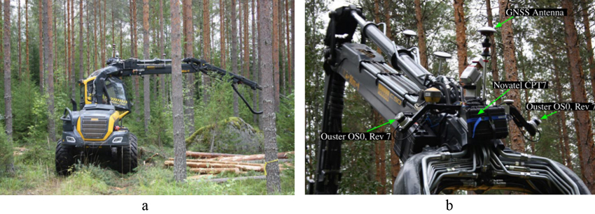
Fig. 1. Study site and the Ponsse Scorpion harvester used for the study (a), and the position of the two Ouster LiDARs, one GNSS antenna, and Novatel CPT7 installed on the boom of the Ponsse harvester (b). The Novatel CPT7 was behind the black box attached to the aluminium frame, not inside the black box.
The harvester LiDAR point cloud data consisted of multiple separate point cloud data files (LAS files), recorded during different sessions of thinning and clear-cutting operations. The point clouds recorded by the Ouster sensors were reconstructed to a global frame using trajectory information obtained using Novatel CPT7 GNSS/INS positioning system. The point cloud densities of harvester LiDAR ranged from 7400 to 20 430 points m–2 within a 30 m of the harvester’s trajectory. All the LiDAR systems used in this study were time-of-flight (ToF) and capable of multi-return measurements, allowing for the detection of multiple surfaces from a single laser pulse. Some important technical features of the LiDAR systems used in this study are presented in Table 1.
| Table 1. Technical specifications of the LiDAR systems used in this study. | |||
| LiDAR system | Lasers wavelength (nm) | Beam radius at exit (mm) | Divergence (mrad) |
| Riegl VUX-1HA | 1550 | 4.5 | 0.5 |
| Riegl VUX-120 | 1550 | NA | 0.4 |
| GeoSLAM Zeb Horizon RT | 903 | 12.7 (horizontal) × 9.5 (vertical) | 3.0 × 1.2, 300 kHz |
| Ouster OS0 (Rev 7) | 865 | 5 | 6 |
2.3 LiDAR data processing
In the preprocessing of LiDAR point clouds (Fig. 2), noise removal (using lasnoise, Isenburg 2019), ground classification (lasground, Isenburg 2019) and height normalization (lasheight, Isenburg 2019), and co-registration of HMLS and harvester LiDAR data to DLS data were performed. The settings for noise removal included a grid resolution of 2 meters in the horizontal plane, a vertical resolution of 1 meter, and points with fewer than 10 neighbors are considered isolated and potentially removed. The Lasground settings included a 2-meter grid step, a 1.5-meter bulge threshold, a spike value of 1, a downspike threshold of 0.3, a 0.05-meter offset, and ultrafine resolution for more precise ground classification. The setting for lasheight we used was to compute height above ground and key points, and to replace Z-values, which produced height-normalized point clouds classified into ground and vegetation points (Fig. 3). The co-registration of HMLS with DLS was conducted using the Iterative Closest Point (ICP) algorithm at 50% overlap on CloudCompare to mitigate possible positional inaccuracies between the different LiDAR systems.
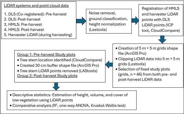
Fig. 2. Workflow for the plot level analysis and comparing consistencies among HMLS, DLS and harvester LiDAR points for low vegetation quantification in this study.
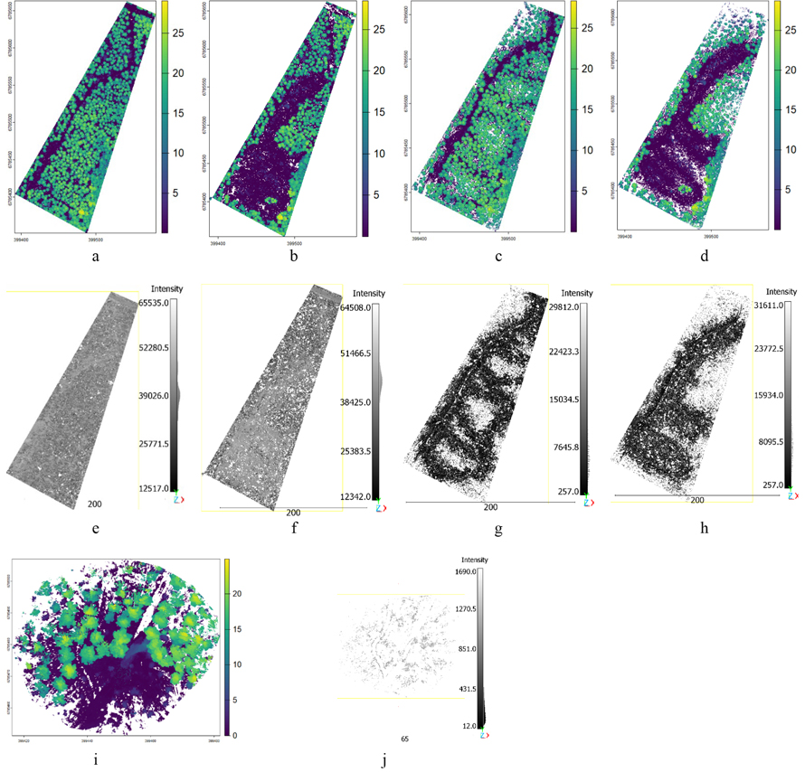
Fig. 3. LiDAR point clouds showing vegetation points (a–d, i) by canopy height and ground points (e–h, j) by intensity values: DLS preharvest (a, e), DLS postharvest (b, f), HMLS preharvest (c, g), HMLS postharvest (d, h), and harvester LiDAR (i, j). View larger in new window/tab.
Registration of HMLS generated cloud points with DLS generated cloud points was conducted using the iterative closest point (ICP) algorithm at 50% overlap on CloudCompare tool to mitigate positional inaccuracies arising from different sensor systems and collection methods. Height normalized DLS cloud points containing the harvested area, and its periphery was segmented and clipped with CloudCompare tool and then processed in ArcGIS Pro to create a 5 m × 5 m grids shapefile (Esri 2024). Individual plots from the LAS files were extracted using the Lasclip function of LAStools tool.
Preprocessing of the harvester LiDAR point cloud data included additional steps as the data was collected continuously during harvesting operation. The main challenge was caused by the lack of clear pre- and post-harvest time points in the continuous flow of point cloud data. Therefore, the harvester’s route (Fig. 4) timestamps (trajectory) and point cloud data from each recording session were first used to identify LiDAR data collected during three harvesting phases: pre-thinning, thinning, and clear-cutting operations. However, to precisely isolate pre- and post-harvest LiDAR data from the harvester, we cross-referenced it with HMLS or DLS point clouds within small, fixed plots (e.g., 25 m2 sample plot).
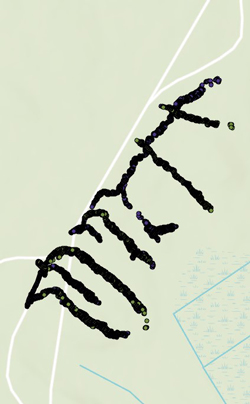
Fig. 4. Harvester trajectory. During the harvesting operations, the trajectory of the harvester was monitored using a robotic total station.
A total of 46 sample plots of 25 m2 were selected (Fig. 5) based on three key criteria. First, all plots were located within 20 meters of the harvester’s trajectory to ensure optimal harvester LiDAR coverage of the forest vegetation structure and to avoid grids with occlusions. Second, each plot had to have both pre- and post-harvest LiDAR data from the harvester that could be accurately matched and compared with the HMLS or DLS datasets. Third, any grid containing point clouds from the harvester itself (considered noise) was excluded from selection. In such cases, an alternative plot without harvester-related point clouds was chosen to maintain data integrity. Then all the different point cloud data were clipped based on the selected sample plot border for further processing separately for (1) pre-harvest and (2) post-harvest (i.e. after clear cutting) point cloud.
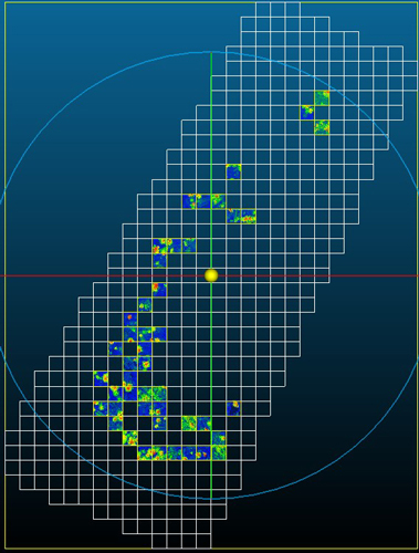
Fig. 5. Harvested area divided into 5 m × 5 m plots (grid cells) and selected plots for study containing point clouds (DLS post-harvest LiDAR point clouds).
The mid-height (5–10 m) and high (>10 m) forest trees (Goodwin et al. 2018) in the pre-harvest LiDAR data were detected and removed from the point cloud, as suggested by Adhikari et al. (2023). Tree stem detection of the dominant trees was performed manually using CloudCompare, as the CloudCompare plugins 3DFin and TreeIso did not perform well with our point clouds. Stem detection in CloudCompare, using intensity-based filtering to isolate stem points, was more accurate than those tools for both our harvester and HMLS LiDAR data. Once the stem point clouds were identified, the stem location (X and Y coordinates) was assigned by using point list picking function of CloudCompare. We created buffers of 20 cm, 25 cm, and 30 cm around each tree location using ArcGIS Pro software (Zhang et al. 2023). We evaluated the effectiveness of different buffer sizes and found that the 25 cm buffer did not successfully remove all stem points in the harvester LiDAR data, while the 30 cm buffer was effective. Therefore, we applied the 30 cm buffer to remove stem point clouds using LAStools (Lasclip and las2las functions). The remaining parts of the stem, for example branches and leaves were removed manually using CloudCompare.
Our tree stem detection and removal method performed well in plots with simple vegetation (only low and high vegetation) but struggled in dense areas containing low, mid-height, and high vegetation. Due to difficulties in distinguishing and removing branches and leaves in mid-height vegetation (even with a 30 cm buffer), we skipped stem removal for mid-height vegetation and treated all mid-height vegetation below 5 m as low vegetation.
The harvester LiDAR point clouds for each plot were processed using Statistical Outlier Removal (SOR) in CloudCompare (k = 6, σ = 1). Selective outlier removal was applied to HMLS data where needed, while DLS data required no such processing. Post-harvest processing was simplified as stem and medium vegetation removal became unnecessary, though harvester LiDAR data still required outlier filtering.
2.4 Quantifying low vegetation attributes
Low vegetation attributes have been quantified in previous studies using various metrics, including height (Sumnall et al. 2017), height percentiles (Friedli et al. 2016; Malambo et al. 2018; Adhikari et al. 2023), and volume (Adhikari et al. 2023; Tienaho et al. 2024). Vegetation density has been assessed using voxel-grid approaches to indicate the presence or absence of vegetation points, as well as through detailed vertical density profiles (Sumnall et al. 2017). Other metrics include cover (Adhikari et al. 2023), plant density index (PDI) profiles for different low vegetation layers such as the forest floor (0.5–1 m), shrubs (1–2 m), and lower understory (2–5 m) (Ferrara et al. 2023), and biomass (Adhikari et al. 2023). For our study, we selected low vegetation attributes related to height variation, volume, and cover as these represent the vertical, three dimensional and horizontal structure of low vegetation. Low vegetation attributes using LiDAR points were estimated using lidR program (Roussel et al. 2024).
2.4.1 Height
Vegetation height, in meters, was determined by removing ground points and calculating the height of vegetation points relative to the ground (height at zero meters) within a plot (Fig. 6a). Height variables such as maximum height, 99th height percentile, 95th height percentile, 90th height percentile, mean height, and median height were calculated. Friedli et al. (2016) demonstrated 99th height percentile with a higher R2 value compared to maximum height between field data and TLS data for height measurement of maize (Zea mays), wheat (Triticum aestivum) and soybean (Glycine max). Similarly, Malambo et al. (2018) reported that 90th, 95th, and 99th height percentiles showed higher correlations compared to maximum height to field measurements of maize and sorghum (Sorghum bicolor). Height percentiles were used in our study because they reduce the effect of noise and outliers, making them more reliable for measuring low vegetation after harvesting trees.
2.4.2 Volume
Volume was calculated by two different methods: mean height and voxel (cubic bin; Fig. 6b) in cubic meter (m3) per plot (25 m2). The mean height-based volume calculation used the mean height of low vegetation in each square bin (grid cell) of three different sizes on each side: 5 cm, 10 cm, and 20 cm. To calculate the total volume, the mean height in each occupied grid (containing at least one vegetation point) was first calculated, and then the volume for each grid was calculated by multiplying its mean height and grid size. The total volume in a plot was calculated by summing the volumes of all occupied grids. As suggested by Adhikari et al. (2023), this method is more accurate for understory biomass calculation compared to the voxel-based and alpha hull methods. Quantification of change in low vegetation by volumetric method using height and grid area (m3 ha–1) was also done in a previous study by Tienaho et al. (2024). Three voxel sizes (5 cm, 10 cm and 20 cm on each side) were fitted to calculate vegetation volume. The total volume in a plot was calculated by summing the volumes of all fitted voxels occupied by low vegetation, as suggested by Enterkine et al. (2025). A voxel was considered occupied if it contained at least one vegetation point. This threshold was adopted because the maximum average number of vegetation points per voxel in some study plots was less than 1.5, 1.5, and 2.5 for voxel sizes of 5 cm, 10 cm, and 20 cm, respectively.
2.4.3 Cover
The same grid sizes as used for volume calculation by mean height method (5 cm, 10 cm, and 20 cm) were employed to calculate low vegetation cover using the canopy height model (CHM) (Fig. 6c) (algorithm: points to raster). Low vegetation cover was calculated by dividing the number of occupied grids in that plot. Since the low vegetation cover is calculated as a ratio, the maximum value is 1 if all the grids are occupied.
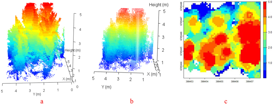
Fig. 6. Visualization of low vegetation structure: Point clouds (a), 10 cm voxels (b), and canopy height with grid size 10 cm (c) (Plot code: Plot 102: harvester LiDAR before harvesting operations).
2.5 Comparison of LiDAR systems: relationships and consistency
This study compared the consistency of harvester LiDAR, HMLS and DLS point clouds for estimating low vegetation attributes through pre- and post-harvest analyses, using the same method for both analyses. DLS data served as the reference for calculating the coefficient of determination (R2) and mean difference (MD) between harvester LiDAR and DLS data, as well as between HMLS and DLS data. However, when comparing harvester LiDAR and HMLS data, HMLS LiDAR data were used as a reference.
To assess statistical differences or similarities among the LiDAR datasets, one-way analysis of variance (ANOVA) or non-parametric tests were conducted based on the results of normality and homogeneity tests. The Shapiro–Wilk test was applied to assess the normality of residuals, with the null hypothesis that the data are normally distributed and the alternative hypothesis that they are not. This test is suitable for small to moderate sample sizes and was used in accordance with Gyawali et al. (2022). Levene’s test was used to assess the homogeneity of variances, assuming under the null hypothesis that all groups have equal variances. Both tests were conducted at a significance level of p < 0.05.
For low vegetation attributes that met both normality and homogeneity criteria (p > 0.05), a one-way ANOVA was performed to test whether there were any statistically significant differences among group means. The null hypothesis for ANOVA is that all group means are equal, while the alternative hypothesis is that at least one group differs. If significant differences were found, Tukey’s honestly significant difference (HSD) post-hoc test was used to identify which pairs of datasets differed.
For attributes where variance was homogeneous, but residuals were not normally distributed, we attempted data transformations (log, square root, or Box-Cox) to meet normality assumptions. These transformations adjust the scale or distribution of the data without changing the relative ranking of values, which can stabilize variance and make the data more suitable for parametric testing. If the transformations failed to achieve normality, we applied the Kruskal–Wallis test, a non-parametric alternative to ANOVA that does not assume normality or equal variances. The null hypothesis for Kruskal–Wallis is that all group medians are equal, and the alternative hypothesis is that at least one group differs. When normality assumptions, or both the normality and homogeneity assumptions were violated (p < 0.05), the Kruskal–Wallis test was also used, followed by Dunn’s post-hoc test to determine which groups differed significantly. Although post-hoc tests are typically used after finding significant differences, Tukey’s HSD and Dunn’s tests were applied here for exploratory purposes across all comparisons.
The maximum height of low vegetation points before harvesting in our study fell into two categories: (1) a maximum height of 5 m, which was derived from a mix of low, mid-height, and high vegetation, and (2) a maximum height below 5 m, which was observed in forest stands containing only low and high vegetation, with no mid-height vegetation. We found that 17 plots contained mid-height vegetation, while 29 plots did not. For the comparison of maximum height using R2 analysis and one-way ANOVA or Kruskal–Wallis tests, we considered only the plots containing low and high vegetation without mid-height vegetation (n = 29). This selection was made to minimize the influence of mid-height trees, where the maximum height was less variable and fixed at 5 m. This approach reduced the risk of bias and ensured that the analysis focused solely on the low vegetation category.
3 Results
3.1 Low vegetation attributes
The maximum vegetation height across all LiDAR datasets was 5 m, reflecting the maximum height limit of low vegetation in the study (Fig. 7a). Before harvesting, the lowest maximum height was 2.94 m (HMLS data), indicating a mix of low and high vegetation but no mid-height vegetation. After harvesting, this value dropped to 0.59 m (DLS data), suggesting that some low trees or shrubs (<5 m) were also removed. The mean maximum height decreased by 1.15–1.23 m due to harvesting.
A similar pattern of reduction was observed in the mean values of the 99th (Fig. 7b), 95th (Fig. 7c), and 90th (Fig. 7d) height percentile across all LiDAR systems. Mean and median heights showed smaller decreases in absolute height (Fig. 7e and Fig. 7f), but larger percentage reductions compared to the higher percentile metrics, highlighting significant changes in low vegetation structure. These consistent declines across all systems confirm the effectiveness of LiDAR in quantifying vegetation height dynamics associated with harvesting activities.
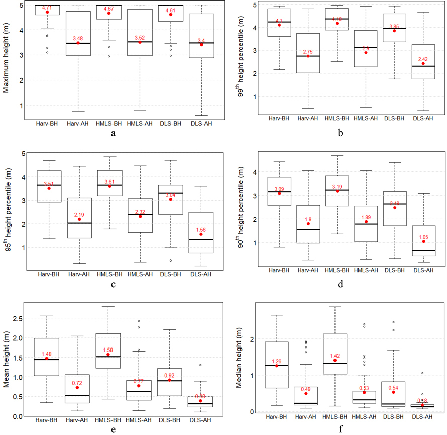
Fig. 7. Low vegetation height metrics (in meters) derived from three LiDAR systems (harvester LiDAR (Harv), HMLS, and DLS) before harvest (BH) and after harvest (AH): (a) maximum height, (b) 99th height percentile, (c) 95th height percentile, (d) 90th height percentile, (e) mean height, and (f) median height. Red points and red numerical values indicate the mean values.
The 20 cm voxels produced the highest low vegetation points occupied volume before harvesting (63.65 m3 by HMLS, Fig. 8f) and after harvesting (49.37 m3 by DLS, Fig. 8f). The lowest volume was recorded with the 5 cm voxel, measuring 0.55 m3 before harvesting and 1.28 m3 after harvesting by DLS (Fig. 8d). Using a 5 cm voxel slightly overestimated post-harvest low vegetation volume compared to pre-harvest for HMLS and DLS. However, for harvester LiDAR, pre-harvest volume is higher than post-harvest at this voxel size (Fig. 8d).
For larger voxel sizes (10 cm and 20 cm, Figs. 8e, 8f) and the mean height-based method (Figs. 8a–c), all three LiDAR systems showed a reduction in low vegetation volume after harvesting. Volume reductions are more consistent across systems when using the mean height-based method (6.8–10.9 m3) compared to the voxel method (0.77–11.79 m3).
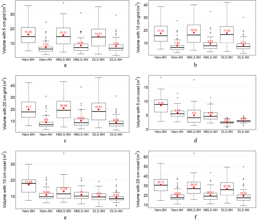
Fig. 8. Low vegetation points-occupied volume metrics (m3 per plot of 25 m2) from three LiDAR systems before and after harvesting. Volumes were estimated using the mean height method with 5 cm (a), 10 cm (b), and 20 cm (c) grids, and by fitting voxels of 5 cm (d), 10 cm (e), and 20 cm (f).
Low vegetation cover ranged from 0.55 to 1 for harvester LiDAR, 0.61 to 1 for HMLS LiDAR, and 0.66 to 1 for DLS LiDAR, indicating a similarity among these LiDAR datasets in estimating vegetation cover and highlighting high vegetation cover based on LiDAR vegetation points (Fig. 9). It was also observed that the low vegetation cover was slightly higher for post-harvest (for harvester LiDAR, HMLS and DLS with 5 cm grid) than for pre-harvest. This could be due to better coverage or improved capture of low vegetation by LiDAR sensors in the absence of trees and in areas with sparse vegetation.
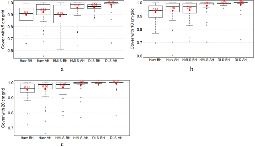
Fig. 9. Low vegetation cover metrics from three LiDAR systems before and after harvesting. Cover was estimated using 5 cm (a), 10 cm (b), and 20 cm grids (c).
3.2 Relationship among LiDAR systems
Maximum height and higher height percentiles (99th, 95th, and 90th) showed strong correlations among LiDAR systems, with R2 values ranging from 0.76 to 0.98, and correlations were stronger post-harvest compared to pre-harvest (Supplementary file S1: Figs. S1a, S1b, S1c, and S1d). Mean height showed moderate to high correlations (R2 0.56–0.88) (Suppl. file S1: Fig. S1d). Weak correlations were found for median height between DLS and HMLS (R2 0.28–0.34); however, there was a moderate correlation between harvester LiDAR and HMLS before harvest (R2 0.57) and a strong correlation after harvest (R2 0.8) (Suppl. file S1: Fig. S1f).
Mean height-based volume estimates exhibited strong correlations before harvesting (R2 0.87–0.93) and remained high post-harvest (R2 0.90–0.98) (Suppl. file S1: Figs. S2a, S2b, and S2c). Volume estimates based on voxels showed poor correlations, especially for 5 cm voxels where R2 ranged from 0.01 to 0.24 (Suppl. file S1: Fig. S2d) before harvesting, improving only slightly post-harvest to 0.56 for 10 cm voxels (Suppl. file S1: Fig. S2e) and 0.83 for 20 cm voxels (Suppl. file S1: Fig. S2f).
Low vegetation cover estimates showed very weak agreement among all three LiDAR systems across all grid sizes and harvest conditions, with R2 values close to zero, except for a slight improvement post-harvest between HMLS and DLS reaching 0.57 (Suppl. file S1: Figs. S3a, S3b, and S3c). These low R2 values indicate very weak linear relationships between LiDAR systems for estimating low vegetation cover.
3.3 Consistencies among LiDAR systems
Only the 90th height percentile preharvest met the normality criteria (W = 0.98, p-value = 0.129). Levene’s test showed that some pre-harvest (volume with 5 cm and 10 cm voxels, cover attributes) and post-harvest attributes (mean height, median height, volume with 5 cm voxel, cover attributes) did not meet the homogeneity of variance criteria and were analyzed using the Kruskal–Wallis test. For attributes that met homogeneity but not normality, data transformation was attempted on 99th height percentile, 95th height percentile, and various volume estimates. Transformation was successful for volume estimated with 20 cm voxels and volume calculated using the mean height method for pre- and post-harvest, as well as post-harvest volume with 10 cm voxels, allowing one way ANOVA test to compare the harvester, HMLS, and DLS LiDAR systems. Attributes that remained non-normal after transformation were analyzed using the Kruskal–Wallis test (Table 2).
The Kruskal–Wallis test results showed that for maximum height and the 99th height percentile, both pre- and post-harvest, there were no significant differences among the three LiDAR systems, indicating high consistency in estimating low vegetation maximum height (p = 0.718 pre-harvest, p = 0.82 post-harvest) and the 99th height percentile (p = 0.149 pre-harvest, p = 0.087 post-harvest). However, for other height attributes (90th height percentile, mean, and median height), significant differences were observed both pre- and post-harvest. The post-hoc tests (Tukey’s HSD for ANOVA and Dunn’s test for the Kruskal–Wallis test) revealed significant differences between DLS and harvester LiDAR, as well as between DLS and HMLS. harvester LiDAR and HMLS consistently estimated all height attributes for both pre- and post-harvest low vegetation, with p-values ranging from 0.25 to 1.
| Table 2. Results of ANOVA and Kruskal–Wallis test on harvester, HMLS and DLS LiDAR for quantifying low vegetation attributes. Test values for one way ANOVA is F-statistic value (F) and for Kruskal–Wallis test Chi-square value (χ2). Short form written in the Test columns: K–W indicate Kruskal–Wallis test, ANOVA indicate one-way ANOVA, and logt, Sqrt, and Box-Cox represent the data transfomation process used to proceeed with one-way ANOVA test. p-values in bold indicate statistical significance (p < 0.05). | ||||||||||||
| Low vegetation attributes | Pre-harvest | Post-harvest | ||||||||||
| Test value | p-value | Adjusted p-value | Test | Test value | p-value | Adjusted p-value | Test | |||||
| Harvester – DLS | HMLS – DLS | HMLS – Harvester | Harvester – DLS | HMLS – DLS | HMLS – Harvester | |||||||
| Maximum height (m) | 0.682 | 0.718 | 0.632 | 0.853 | 1.000 | K–W | 0.405 | 0.820 | 1.000 | 0.796 | 1.000 | K–W |
| 99th height percentile (m) | 3.809 | 0.149 | 0.320 | 0.081 | 0.744 | K–W | 4.863 | 0.087 | 0.198 | 0.047 | 0.779 | K–W |
| 95th height percentile (m) | 8.948 | 0.011 | 0.037 | 0.006 | 0.825 | K–W | 11.870 | 0.0026 | 0.0096 | 0.0021 | 0.960 | K–W |
| 90th height percentile (m) | 8.138 | 0.0004 | 0.004 | 0.0008 | 0.855 | ANOVA | 18.570 | 9.25e-05 | 0.0005 | 0.0002 | 1.000 | K–W |
| Mean height (m) | 19.75 | 3.01e-08 | 0.0000 | 0.0000 | 0.716 | Box-Cox | 21.810 | 1.83e-05 | 0.0004 | 0.0000 | 0.771 | K–W |
| Median height (m) | 39.092 | 3.24e-09 | 0.0000 | 0.0000 | 0.669 | K–W | 40.517 | 1.59e-09 | 0.0000 | 0.0000 | 0.250 | K–W |
| Volume with 5 cm grid (m3) | 0.721 | 0.488 | 0.500 | 0.624 | 0.978 | Sqrt | 0.984 | 0.377 | 0.816 | 0.708 | 0.344 | logt |
| Volume with 10 cm grid (m3) | 0.058 | 0.943 | 0.999 | 0.948 | 0.958 | Sqrt | 1.343 | 0.264 | 0.951 | 0.428 | 0.273 | Box-Cox |
| Volume with 20 cm grid (m3) | 0.209 | 0.812 | 0.959 | 0.795 | 0.927 | logt | 1.611 | 0.204 | 0.980 | 0.232 | 0.317 | Box-Cox |
| Volume with 5 cm voxel (m3) | 75.229 | 2.2e-16 | 0.0000 | 0.0001 | 0.0000 | K–W | 66.027 | 4.59e-15 | 0.0000 | 0.0000 | 0.058 | K–W |
| Volume with 10 cm voxel (m3) | 38.793 | 3.76e-09 | 0.0000 | 0.0132 | 0.0005 | K–W | 4.618 | 0.0115 | 0.036 | 0.018 | 0.966 | Box-Cox |
| Volume with 20 cm voxel (m3) | 2.674 | 0.072 | 0.059 | 0.613 | 0.366 | logt | 0.755 | 0.472 | 0.993 | 0.507 | 0.573 | Box-Cox |
| Cover with 5 cm grid | 18.511 | 9.55e-05 | 0.0001 | 0.0010 | 0.846 | K–W | 42.358 | 6.33e-10 | 0.0000 | 0.0003 | 0.0085 | K–W |
| Cover with 10 cm grid | 47.828 | 4.11e-11 | 0.0000 | 0.0000 | 0.079 | K–W | 48.547 | 2.87e-11 | 0.0000 | 0.0021 | 0.0003 | K–W |
| Cover with 20 cm grid | 48.470 | 2.97e-11 | 0.0000 | 0.0000 | 0.025 | K–W | 42.812 | 5.05e-10 | 0.0000 | 0.082 | 0.0000 | K–W |
Consistency among the three LiDAR systems was observed in estimating low vegetation volume using the mean height method with 5 cm, 10 cm, and 20 cm grids, as well as in volume estimations using large voxels (20 cm) for both pre- and post-harvest low vegetation (Table 2). However, there was no consistency among the three LiDAR systems in estimating pre-harvest low vegetation volume using smaller voxels (5 cm and 10 cm). The post-hoc analyses, using Dunn’s test for the Kruskal–Wallis test and Tukey’s HSD for ANOVA, yielded varying results depending on the voxel size used to calculate post-harvest low vegetation volume. At the 10 cm voxel resolution, the p-value was 0.966, indicating no statistically significant difference between harvester LiDAR and HMLS. At the 5 cm resolution, the p-value was 0.058, which also does not meet the threshold for statistical significance but is close to the conventional cutoff of 0.05. Although both voxel sizes showed no statistically significant differences, the 5 cm result should be interpreted with greater caution due to its proximity to the significance threshold, which may suggest a potential trend or sensitivity to data variability.
The Kruskal–Wallis test results indicated a very high significant difference among the LiDAR systems in estimating low vegetation cover for both pre- and post-harvest (p < 0.0001). Dunn’s post-hoc test for the Kruskal–Wallis analysis revealed that harvester LiDAR and HMLS were consistent in estimating low vegetation cover at smaller resolutions (5 cm and 10 cm, p-values: 0.846 and 0.079, respectively) for pre-harvest. Additionally, consistency was observed between HMLS and DLS for estimating low vegetation cover at higher resolutions (20 cm grid, p-value 0.082). Post-hoc tests from Kruskal–Wallis or ANOVA indicated general consistency between LiDAR systems in estimating low vegetation cover and volume using the voxel method; however, the corresponding R2 values were low and inconsistent. For example, high consistency between the harvester and HMLS systems before harvesting for estimating cover using a 5 cm grid (p = 0.846) corresponded with a very low R2 value (R2 0.05) (Suppl. file S1: Fig. S3a). Similarly, for the 10 cm grid, which also showed consistency (p = 0.079), the R2 value was only 0.08 (Suppl. file S1: Fig. S3b). For the cover estimated using 20 cm grid after harvest, the comparison between HMLS and DLS resulted in an R2 of 0.57 (Suppl. file S1: Fig. S3a), with a p-value of 0.082 (Table 2) indicating consistency. A very high consistency was observed between HMLS and harvester for estimating volume using a 10 cm voxel size after harvest (p = 0.966), yet the R2 value was moderate (R2 0.52) (Suppl. file S1: Fig. S2e). For the 5 cm voxel size, the R2 was 0.24 (Suppl. file S1: Fig. S2d) despite a relatively consistent result (p = 0.058) (Table 2). These findings suggest that although there is statistical agreement at the group level, voxel-based and cover-based estimates, particularly at finer resolutions, have limited ability to explain variability across LiDAR systems.
In summary, harvester LiDAR, HMLS, and DLS demonstrated consistency in estimating low vegetation maximum height, volume calculated using a 20 cm voxel, and volume calculated using the mean height and cover methods with 5 cm, 10 cm, and 20 cm grids.
4 Discussion
Quantifying the vegetation characteristics using LiDAR technology requires careful consideration of several important factors, including the selection of reference data, standardized methodology, appropriate LiDAR metrics (Campbell et al. 2018; Adhikari et al. 2023), and explanatory variables (Adhikari et al. 2023; Enterkine et al. 2023), all of which we considered in our study. We selected DLS and HMLS (rather than field data) for comparison with harvester LiDAR due to their non-destructive sampling advantages and widespread use in forest inventory as ALS has shown higher precision for structure, cover, and maximum height (Sumnall et al. 2017; Venier et al. 2019) of low vegetation. MLS applications for low vegetation remain limited but are well-established for forest inventory and understory trees (Lin et al. 2014) and excels in DBH measurement (Hyyppä et al. 2020; Stal et al. 2021; Vatandaşlar and Zeybek 2021) and used for below-canopy structural attribute extraction (Ryding et al. 2015) and individual tree mapping (Tupinambá-Simões et al. 2023).
To achieve our study objectives, we quantified low vegetation characteristics including height, volume, and cover through an area-based grid processing of point cloud data. To understand harvesting impacts on low vegetation, we compared these vegetation metrics before and after clear-cutting operations. Furthermore, we systematically evaluated the performance consistency between harvester LiDAR, HMLS, and DLS systems for estimating low vegetation parameters.
It is not logical to directly compare our results on quantified low vegetation attributes with those from previous studies, as low vegetation characteristics vary between forest stands due to factors such as vegetation condition, the maximum height threshold considered, estimation method and the defining criteria of low vegetation based on study objectives. This is particularly evident in volume estimates, where different methods yield varying results. In our study, we did not consider the stems of dominant trees (high vegetation) as low vegetation. In contrast, Tienaho et al. (2024) included tree stems in their assessment of fire-induced ground vegetation changes (vegetation <2 m). Adhikari et al. (2023) reported that different methods with varying resolutions produced different volume estimates for the same plot. While we acknowledge these methodological differences, our focus is not on the absolute quantity of volume estimated but rather on the comparative patterns of estimation between voxel-based and mean height-based approaches. Our findings revealed both consistency and discrepancies with their results. Adhikari et al. (2023) reported that the highest mean volume was obtained using a 20 cm voxel, followed by the mean height method (20 cm grid), then the 10 cm grid, and finally the 10 cm voxel, which yielded the lowest volume. Our study aligned with theirs in that the 20 cm voxel produced the highest mean volume. However, the pattern diverges in that the lowest volume in our case was estimated using either the 10 cm voxel or the 10 cm grid, depending on LiDAR type and pre- or post-harvest conditions. These differences may stem from variations in vegetation structure, plot size, and LiDAR systems. Adhikari et al. (2023) analyzed low vegetation up to 3 m in height within a well-managed pine forest in Florida, USA, using TLS in 1 m × 1 m subplots. In contrast, our study considered vegetation up to 5 m in a mixed boreal forest, with larger 5 m × 5 m plots, which likely contributed to the observed discrepancies.
A key limitation of voxelization is the risk of volume overestimation when voxels are considered occupied based on just one or a few points, especially in sparse vegetation and with larger voxel sizes. To address this issue, we employed relatively small voxel resolutions (5 cm, 10 cm, and 20 cm) and established a minimum point threshold to determine voxel occupancy. In our study, pre-harvest data in certain plots exhibited low point densities, with fewer than two vegetation points per voxel for the 5 cm and 10 cm sizes, and fewer than 2.5 points for the 20 cm voxels. We adopted a conservative threshold of one point per voxel to define occupancy. While this criterion may have introduced some degree of overestimation, it provided a consistent basis for comparison. Future research could enhance volume estimation accuracy by implementing more sophisticated approaches, such as adaptive point thresholds or alternative metrics suited for low-density vegetation and understory characterization beneath dense canopy cover.
After quantifying low vegetation characteristics, this study assessed the consistency among three LiDAR systems in measuring low vegetation before and after harvest. We assessed agreement and discrepancies using the coefficient of determination (R2), mean difference values, one-way ANOVA, and the Kruskal–Wallis test. The harvester LiDAR data showed both agreements and discrepancies with HMLS and DLS in estimating low vegetation attributes. For height variables such as maximum height and the 99th height percentile, results were consistent across the systems. Similarly, volume estimation using the mean height method and higher voxel size (20 cm) also demonstrated consistency. Previous studies support the effectiveness of volume-based metrics (e.g., voxel-based and mean height-based approaches) for low vegetation volume and biomass estimation. Adhikari et al. (2023) reported that the mean height-based volumetric method at 10 cm resolution had the highest predictability (adjusted R2 0.80), followed by 20 cm resolution (adjusted R2 0.78). In contrast, Cooper et al. (2017) observed lower prediction accuracy (R2 0.42–0.54) using a mean height and area-based method. Enterkine et al. (2023) revealed that voxel sizes of 0.5 cm best represented biomass (R2 0.42), while Li et al. (2021) demonstrated high predictability (R2 0.69) for shrub biomass using a mean height-based method. This study did not explore comparisons between voxel-based and mean-height-based volume metrics in terms of their strengths, limitations, and suitability for specific research objectives. Nevertheless, findings from both this study and Adhikari et al. (2023) suggest that volume is significantly influenced by voxel size than by grid size in the mean-height method. This presents another area for future investigation, particularly in optimizing volume metrics for low vegetation analysis.
Post-hoc test results of our study indicated that harvester LiDAR aligned with HMLS in estimating other height variables (95th height percentile, 90th height percentile), voxel-based volume (post-harvest), and cover attribute relationships not observed between harvester LiDAR and DLS or between HMLS and DLS. This suggests that harvester LiDAR and HMLS are comparable for estimating low vegetation attributes. However, despite a consistent relationship (p > 0.05) between harvester LiDAR and HMLS, low R2 values (<0.1) indicate a non-normal distribution of vegetation LiDAR points and a non-linear relationship between the two systems, as the coefficient of determination (R2) primarily quantifies the strength of linear relationships (Pennsylvania State University 2018).
Our study faced specific challenges in point cloud processing and low vegetation detection, presenting opportunities for further research and methodological improvements. Rather than directly identifying low vegetation, which is inherently difficult as noted by Huo et al. (2022), we adopted an approach based on detecting medium and high vegetation by their stems and removing them using a 30 cm linear buffer, as suggested by Zhang et al. (2023). Huo et al. (2022) partially addressed this issue through their Symmetrical Structure Detection (SSD) algorithm, which successfully separated overstory and understory LiDAR points. However, their study excluded vegetation below 1 m due to validation constraints, whereas our research considers all vegetation under 5 m. This methodological difference highlights a persistent gap in low vegetation detection frameworks and underscores a promising avenue for future studies. Additionally, the complex vegetation structure comprising low, medium, and high strata posed a significant challenge in completely removing medium vegetation, including branches and leaves, without inadvertently eliminating low vegetation point clouds. As outlined in our methodology, this limitation necessitated distinct processing approaches for medium and high vegetation. While a unified method for both categories would have been ideal, practical constraints made this infeasible. Addressing these issues in future studies could lead to more refined methodologies for low vegetation detection in complex forest environments.
Another challenge in data processing arose from the limitations of the harvester LiDAR, particularly when handling over 600 LAS files due to the system’s limited range. While effective within 15 m of its trajectory, point density declined markedly beyond 20 m (Faitli et al. 2024), necessitating labor-intensive manual processing. Future improvements should focus on extending LiDAR range to enhance data accuracy for distant vegetation and developing automated processing techniques to boost efficiency. Addressing these gaps could refine low vegetation detection methods, advancing forest monitoring and management practices.
5 Conclusion
This study demonstrated the reliable performance of harvester-mounted LiDAR compared to handheld and drone-based systems in accurately estimating key low vegetation attributes using area-based point cloud processing techniques. These attributes include maximum height, the 99th height percentile, and volume derived using the mean height and cover methods, particularly at smaller grid sizes (5 cm, 10 cm, and 20 cm) and with 20 cm voxel resolution. Inconsistencies appeared for other low vegetation metrics, such as cover estimated with 5 cm, 10 cm, and 20 cm grids, volume calculated using smaller voxels (5 cm and 10 cm), and height metrics including the 90th and 95th percentiles, mean height, and median height. Consistent results underscore the potential to integrate harvester-mounted LiDAR into routine forestry operations for efficient and accurate low vegetation assessment. Accurate quantification of low vegetation using this technology offers valuable opportunities to support sustainable harvesting practices, enhance wildlife habitat identification, and contribute to biodiversity conservation by providing precise data on key indicators such as dense vegetation patches favoured by game species.
Authors’ contributions
Conceptualization (BK; VK; HK; KV; KK), raw data processing (AK; HK; TF), data processing and analysis (BK; VK; HK; KV; KK), writing – original draft preparation (BK), visualization (BK), writing – review and editing (All). All authors have read and agreed to the published version of the manuscript.
Acknowledgments
The authors gratefully acknowledge the Häme University of Applied Sciences, Evo Campus, in particular Esa Lientola and Juha Mäkelä, for their invaluable cooperation in test site selection, usage, and field test arrangements. The ScanForest research infrastructure is also acknowledged.
Funding
The “IlmoStar” project (VN/27353/2022), funded by the Ministry of Agriculture and Forestry in Finland and the European Union’s Next Generation EU program, provided funding for the author’s doctoral program in Science, Forestry, and Technology (LUMETO) at the University of Eastern Finland. This project was coordinated by FGI, with UEF, Luke, and Ponsse Plc as its partners. The IlmoStar project is a part of the UNITE Flagship.
Declaration of openness of research materials, data, and code
The data are available upon request from Binod Kafle or through the open research repository https://doi.org/10.5281/zenodo.16785717.
References
Adhikari A, Peduzzi A, Monter CR, Osborne N, Mishra DR (2023) Assessment of understory vegetation in a plantation forest of the southeastern United States using terrestrial laser scanning. Ecol Inform 77, article id 102254. https://doi.org/10.1016/j.ecoinf.2023.102254.
Balandier P, Gobin R, Prévosto B, Korboulewsky N (2022) The contribution of understorey vegetation to ecosystem evapo-transpiration in boreal and temperate forests: a literature review and analysis. Eur J For Res 141: 979–997. https://doi.org/10.1007/s10342-022-01505-0.
Bienert A, Georgi L, Kunz M, Maas H-G, Von Oheimb G (2018) Comparison and combination of mobile and terrestrial laser scanning for natural forest inventories. Forests 9, article id 395. https://doi.org/10.3390/f9070395.
Boch S, Berlinger M, Fischer M, Knop E, Nentwig W, Türke M, Prati D (2013) Fern and bryophyte endozoochory by slugs. Oecologia 172: 817–822. https://doi.org/10.1007/s00442-012-2536-0.
Campbell MJ, Dennison PE, Hudak AT, Parham LM, Butler BW (2018) Quantifying understory vegetation density using small-footprint airborne lidar. Remote Sens Environ 215: 330–342. https://doi.org/10.1016/j.rse.2018.06.023.
CloudCompare, Version 2.6.3 (2024). https://cloudcompare-org.danielgm.net/release/. Accessed 1 March 2024.
Cooper SD, Roy DP, Schaaf CB, Paynte I (2017) Examination of the potential of terrestrial laser scanning and structure-from-motion photogrammetry for rapid nondestructive field measurement of grass biomass. Remote Sens 9, article id 531. https://www.mdpi.com/2072-4292/9/6/531.
Donager JJ, Sánchez Meador AJ, Blackburn RC (2021) Adjudicating perspectives on forest structure: how do airborne, terrestrial, and mobile lidar-derived estimates compare? Remote Sens 13, article id 2297. https://doi.org/10.3390/rs13122297.
Elliott KJ, Vose JM, Knoepp JD, Clinton BD, Kloeppel BD (2015) Functional role of the herbaceous layer in eastern deciduous forest ecosystems. Ecosystems 18: 221–236. https://doi.org/10.1007/s10021-014-9825-x.
Enterkine J, Hojatimalekshah A, Vermillion M, Van Der Weide T, Arispe SA, Price WJ, Hulet A, Glenn NF (2025) Voxel volumes and biomass: estimating vegetation volume and litter accumulation of exotic annual grasses using automated ultra-high-resolution SfM and advanced classification techniques. Ecol Evol 15, article id e70883. https://doi.org/10.1002/ece3.70883.
Eriksson HM, Eklundh L, Kuusk A, Nilson T (2006) Impact of understory vegetation on forest canopy reflectance and remotely sensed LAI estimates. Remote Sens Environ 103: 408−418. https://doi.org/10.1016/j.rse.2006.04.005.
Eskelson BNI, Madsen L, Hagar JC, Temesgen H (2011) Estimating riparian understory vegetation cover with beta regression and copula models. For Sci 57: 212–221. https://doi.org/10.1093/forestscience/57.3.212.
Esri (2024) ArcGIS Pro. https://www.esri.com/en-us/arcgis/products/arcgis-pro/overview. Accessed 1 March 2024.
Faitli T, Hyyppä E, Hyyti H, Hakala T, Kaartinen H, Kukko A, Muhojoki J, Hyyppä J (2024) Integration of a mobile laser scanning system with a forest harvester for accurate localization and tree stem measurements. Remote Sens 16, article id 3292. https://doi.org/10.3390/rs16173292.
Ferrara C, Puletti N, Guasti M, Scotti R (2023) Mapping understory vegetation density in mediterranean forests: insights from airborne and terrestrial laser scanning integration. Sensors 23, article id 511. https://doi.org/10.3390/s23010511.
Frankenstein S, Koenig G (2004) FASST vegetation models. U.S. Army Engineer Research and Development Center/Cold Regions Research and Engineering Laboratory, Washington DC, ERDC/CRREL TR-04-25. https://www.arlis.org/docs/vol1/74274930.pdf. Accessed 1 March 2024.
Friedli M, Kirchgessner N, Grieder C, Liebisch F, Mannale M, Walter A (2016) Terrestrial 3D laser scanning to track the increase in canopy height of both monocot and dicot crop species under field conditions. Plant Methods 12, article id 9. https://doi.org/10.1186/s13007-016-0109-7.
Fu LT (2019) Potential differences in seed dispersals of low‐height vegetation between single element and windbreak‐like clumps. Ecol Evol 9: 12639–12648. https://doi.org/10.1002/ece3.5727.
George LO, Bazzaz FA (2014) The herbaceous layer as a filter determining spatial pattern in forest tree regeneration. In: Gillam F (ed) The herbaceous layer in forests of eastern North America, New York, NY. Oxford University Press, pp 340–355. https://doi.org/10.1093/acprof:osobl/9780199837656.003.0014.
GeoSLAM Ltd (2022) ZEB Horizon RT: hardware user guide. https://download.faro.com/ui/core/index.html?mode=public&referrer=%2Furl%2Ffcd2yb2tttku3ffb#expl-tabl./SHARED/%211XsXFn8FQFxEp/HtGYqPL3JFhJM5oY. Accessed 11 November 2024.
Gollob C, Ritter T, Nothdurft A (2020). Forest inventory with long range and high-speed Personal Laser Scanning (PLS) and Simultaneous Localization and Mapping (SLAM) technology. Remote Sens 12, article id 1509. https://doi.org/10.3390/rs12091509.
Goodwin CED, Hodgson DJ, Bailey S, Bennie J, McDonald RA (2018) Habitat preferences of hazel dormice Muscardinus avellanarius and the effects of tree-felling on their movement. Forest Ecol Manag 427: 190–199. https://doi.org/10.1016/j.foreco.2018.03.035.
Gyawali A, Aalto M, Peuhkurinen J, Villikka M, Ranta T (2022) Comparison of individual tree height estimated from lidar and digital aerial photogrammetry in young forests. Sustainability 14, article id 3720. https://doi.org/10.3390/su14073720.
Hartley RJL, Jayathunga S, Massam PD, De Silva D, Estarija HJ, Davidson SJ, Wuraola A, Pearse GD (2022) Assessing the potential of backpack-mounted mobile laser scanning systems for tree phenotyping. Remote Sens 14, article id 3344. https://doi.org/10.3390/rs14143344.
Huffman DW, Laughlin DC, Pearson KM, Pandey S (2009) Effects of vertebrate herbivores and shrub characteristics on arthropod assemblages in a northern Arizona forest ecosystem. Forest Ecol Manag 258: 616–625. https://doi.org/10.1016/j.foreco.2009.04.025.
Hunčaga M, Chudá J, Tomaštík J, Slámová M, Koreň M, Chudý F (2020) The comparison of stem curve accuracy determined from point clouds acquired by different terrestrial remote sensing methods. Remote Sens 12, article id 2739. https://doi.org/10.3390/rs12172739.
Huo L, Lindberg E, Holmgren J (2022) Towards low vegetation identification: a new method for tree crown segmentation from LiDAR data based on a symmetrical structure detection algorithm (SSD). Remote Sens Environ 270, article id 112857. https://doi.org/10.1016/j.rse.2021.112857.
Hyyppä E, Yu X, Kaartinen H, Hakala T, Kukko A, Vastaranta M, Hyyppä J (2020) Comparison of backpack, handheld, under-canopy UAV, and above-canopy UAV laser scanning for field reference data collection in boreal forests. Remote Sens 12, article id 3327. https://doi.org/10.3390/rs12203327.
Isenburg M (2019) LAStools – efficient LiDAR processing software, version 2019, academic license). https://rapidlasso.com/lastools/. Accessed 1 March 2024.
Jaakkola A, Hyyppä J, Kukko A, Yu X, Kaartinen H, Lehtomäki M, Lin Y (2010) A low-cost multi-sensoral mobile mapping system and its feasibility for tree measurements. ISPRS J Photogramm 65: 514–522. https://doi.org/10.1016/j.isprsjprs.2010.08.002.
Jones CE, Van Dongen A, Aubry J, Schreiber SG, Degenhardt D (2022) Use of mobile laser scanning (MLS) to monitor vegetation recovery on linear disturbances. Forests 13, article id 1743. https://doi.org/10.3390/f13111743.
Kärhä K (2006) Effect of undergrowth on the harvesting of first-thinning wood. For Stud 45: 101–117.
Kärhä K, Bergström D (2020) Assessing the guidelines for pre-harvest clearing operations of understorey in first thinnings: preliminary results from Stora Enso in Finland. Eur J For Eng 6: 14–22. https://doi.org/10.33904/ejfe.645639.
Korhonen L, Kärhä K, Maltamo M, Malinen J, Hyyppä J, Kaartinen H, Toivonen J, Packalen P, Koivula M (2024) Kaukokartoitus ja metsäkoneiden sensorit metsien monimuotoisuusindikaattorien seurannassa. [Remote sensing and forest machine sensors in monitoring forest biodiversity indicators]. Metsätieteen aikakauskirja, article id 23010. https://doi.org/10.14214/ma.23010.
Kukko A, Kaijaluoto R, Kaartinen H, Lehtola VV, Jaakkola A, Hyyppä J (2017) Graph SLAM correction for single scanner MLS forest data under boreal forest canopy. ISPRS J Photogramm 132: 199–209. https://doi.org/10.1016/j.isprsjprs.2017.09.006.
Kuzmin A, Korhonen L, Kivinen S, Hurskainen P, Korpelainen P, Tanhuanpää T, Maltamo M, Vihervaara P, Kumpula T (2021) Detection of European Aspen (Populus tremula L.) based on an unmanned aerial vehicle approach in boreal forests. Remote Sens 13, article id 1723. https://doi.org/10.3390/rs13091723.
Landuyt D, De Lombaerde E, Perring MP, Hertzog LR, Ampoorter E, Maes SL, De Frenne P, Ma S, Proesmans W, Blondeel H, Sercu BK, Wang B, Wasof S, Verheyen K (2019) The functional role of temperate forest understorey vegetation in a changing world. Global Change Biol 25: 3625–3641. https://doi.org/10.1111/gcb.14756.
Li S, Wang T, Hou Z, Gong Y, Feng L, Ge J (2021) Harnessing terrestrial laser scanning to predict understory biomass in temperate mixed forests. Ecol Indic 121: 1–11. https://doi.org/10.1016/j.ecolind.2020.107011.
Lin Y, Holopainen M, Kankare V, Hyyppä J (2014) Validation of mobile laser scanning for understory tree characterization in urban forest. IEEE J Sel Top Appl 7: 3167–3173. https://doi.org/10.1109/JSTARS.2013.2295821.
Ma T, Zhang C, Ji L, Zuo Z, Beckline M, Hu Y, Li X, Xiao X (2024) Development of forest aboveground biomass estimation, its problems and future solutions: a review. Ecol Indic 159, article id 111653. https://doi.org/10.1016/j.ecolind.2024.111653.
Malambo L, Popescu SC, Murray SC, Putman E, Pugh NA, Horne DW, Richardson G, Sheridan R, Rooney WL, Avant R, Vidrine M, McCutchen B, Baltensperger D, Bishop M (2018) Multitemporal field-based plant height estimation using 3D point clouds generated from small unmanned aerial systems high-resolution imagery. Int J Appl Earth Obs Geoinf 64: 31–42. https://doi.org/10.1016/j.jag.2017.08.014.
Muhojoki J, Tavi D, Hyyppä E, Lehtomäki M, Faitli T, Kaartinen H, Kukko A, Hakala T, Hyyppä J (2024) Benchmarking under- and above-canopy laser scanning solutions for deriving stem curve and volume in easy and difficult boreal forest conditions. Remote Sens 16, article id 1721. https://doi.org/10.3390/rs16101721.
Muller RN (2014) Nutrient relations of the herbaceous layer in deciduous forest ecosystems. In: Gilliam F (ed) The herbaceous layer in forests of eastern North America, New York, NY. Oxford University Press, pp 12–34. https:/doi.org/10.1093/acprof:osobl/9780199837656.003.0002.
Nardinocchi C, Esposito S (2024) Filtering of point clouds acquired by mobile laserscanner for digital terrain model generation indensely vegetated green architectures. Photogram Rec 40, article id e12525. https://doi.org/10.1111/phor.12525.
Ouster (2024) OS0 ultra-wide view high-resolution imaging lidar. https://data.ouster.io/downloads/datasheets/datasheet-rev7-v3p1-os0.pdf. Accessed 11 November 2024.
Penman S, Lentini P, Law B, York A (2023) An instructional workflow for using terrestrial laser scanning (TLS) to quantify vegetation structure for wildlife studies. Forest Ecol Managem 548, article id 121405. https://doi.org/10.1016/j.foreco.2023.121405.
Pennsylvania State University (2018) Lesson 2: Simple Linear Regression (SLR) model. 2.8 - R-squared cautions. Penn State Eberly College of Science, Applied Regression Analysis, STAT 462. https://online.stat.psu.edu/stat462/node/98/. Accessed 4 March 2025.
Riegl (2024) Riegl VUX-12023. http://www.riegl.com/uploads/tx_pxpriegldownloads/RIEGL_VUX-120-23_Datasheet_2024-09-06.pdf. Accessed 11 November 2024.
Roussel J-R, Goodbody TRH, Tompalski P (2024) The lidR package. https://r-lidar.github.io/lidRbook/. Accessed 15 January 2024.
Ryding J, Williams E, Smith MJ, Eichhorn MP (2015) Assessing handheld mobile laser scanners for forest surveys. Remote Sens 7: 1095–1111. https://doi.org/10.3390/rs70101095.
Sagar A, Kärhä K, Einola K, Koivusalo A (2024) Assessing the potential of onboard LiDAR-based application to detect the quality of tree stems in Cut-to-Length (CTL) harvesting operations. Forests 15, article id 818. https://doi.org/10.3390/f15050818.
Song J, Zhu X, Qi J, Pang Y, Yang L, Yu L (2021) A method for quantifying understory leaf area index in a temperate forest through combining small footprint full-waveform and point cloud LiDAR data. Remote Sens 13, article id 3036. https://doi.org/10.3390/rs13153036.
Stal C, Verbeurgt J, De Sloover L, De Wulf A (2021) Assessment of handheld mobile terrestrial laser scanning for estimating tree parameters. J For Res 32: 1503–1513. https://doi.org/10.1007/s11676-020-01214-7.
Stovall AEL, MacFarlane DW, Crawford D, Jovanovic T, Frank J, Brack C (2023) Comparing mobile and terrestrial laser scanning for measuring and modelling tree stem taper. Forestry 96: 705–717. https://doi.org/10.1093/forestry/cpad012.
Sumnall M, Fox TR, Wynne RH, Thomas VA (2017) Mapping the height and spatial cover of features beneath the forest canopy at small-scales using airborne scanning discrete return Lidar. ISPRS J Photogramm 133: 186–200. https://doi.org/10.1016/j.isprsjprs.2017.10.002.
Szostak M, Pająk M (2023) LiDAR point clouds usage for mapping the vegetation cover of the “Fryderyk” mine repository. Remote Sens 15, article id 201. https://doi.org/10.3390/rs15010201.
Thrippleton T, Bugmann H, Folini M, Snell RS (2018) Overstorey–understorey interactions intensify after drought-induced forest die-off: long-term effects for forest structure and composition. Ecosystems 21: 723–739. https://doi.org/10.1007/s10021-017-0181-5.
Tienaho N, Saarinen N, Yrttimaa T, Kankare V, Vastaranta M (2024) Quantifying fire-induced changes in ground vegetation using bitemporal terrestrial laser scanning. Silva Fenn 58, article id 23061. https://doi.org/10.14214/sf.23061.
Torralba J, Carbonell-Rivera JP, Ruiz LÁ, Crespo-Peremarch P (2022) Analyzing TLS scan distribution and point density for the estimation of forest stand structural parameters. Forests 13, article id 2115. https://doi.org/10.3390/f13122115.
Torresan C, Berton A, Carotenuto F, Di Gennaro SF, Gioli B, Matese A, Miglietta F, Vagnoli C, Zaldei A, Wallace L (2017) Forestry applications of UAVs in Europe: a review. Int J Remote Sens 38: 2427–2447. https://doi.org/10.1080/01431161.2016.1252477.
Tuanmu M-N, Viña A, Bearer S, Xu W, Ouyang Z, Zhang H, Liu J (2010) Mapping understory vegetation using phenological characteristics derived from remotely sensed data. Remote Sens Environ 114: 1833–1844. https://doi.org/10.1016/j.rse.2010.03.008.
Tupinambá-Simões F, Pascual A, Guerra-Hernández J, Ordóñez C, de Conto T, Bravo F (2023) Assessing the performance of a handheld laser scanning system for individual tree mapping – a mixed forests showcase in Spain. Remote Sens 15, article id 1169. https://doi.org/10.3390/rs15051169.
Vatandaşlar C, Zeybek M (2021) Extraction of forest inventory parameters using handheld mobile laser scanning: a case study from Trabzon, Turkey. Measurement 177, article id 109328. https://doi.org/10.1016/j.measurement.2021.109328.
Venier LA, Swystun T, Mazerolle MJ, Kreutzweiser DP, Wainio-Keizer KL, McIlwrick KA, Woods ME, Wang X (2019) Modelling vegetation understory cover using LiDAR metrics. PLoS ONE 14, article id e0220096. https://doi.org/10.1371/journal. pone.0220096.
Yang X, Qiu S, Zhu Z, Rittenhouse C, Riordan D, Cullerton M (2023) Mapping understory plant communities in deciduous forests from Sentinel-2 time series. Remote Sens Environ 293, article id 113601. https://doi.org/10.1016/j.rse.2023.113601.
Zhang Y, Tan Y, Onda Y, Hashimoto A, Gomi T, Chiu C, Inokoshi S (2023) A tree detection method based on trunk point cloud section in dense plantation forest using drone LiDAR data. For Ecosyst 10, article id 100088. https://doi.org/10.1016/j.fecs.2023.100088.
Total of 66 references.
