Sakari Tuominen  ,
Andras Balazs,
Eija Honkavaara,
Ilkka Pölönen,
Heikki Saari,
Teemu Hakala,
Niko Viljanen
,
Andras Balazs,
Eija Honkavaara,
Ilkka Pölönen,
Heikki Saari,
Teemu Hakala,
Niko Viljanen
Hyperspectral UAV-imagery and photogrammetric canopy height model in estimating forest stand variables
Tuominen S., Balazs A., Honkavaara E., Pölönen I., Saari H., Hakala T., Viljanen N. (2017). Hyperspectral UAV-imagery and photogrammetric canopy height model in estimating forest stand variables. Silva Fennica vol. 51 no. 5 article id 7721. https://doi.org/10.14214/sf.7721
Highlights
- Hyperspectral imagery and photogrammetric 3D point cloud based on RGB imagery were acquired under weather conditions changing from cloudy to sunny
- Calibration of hyperspectral imagery was required for compensating the effect of varying weather conditions
- The combination of hyperspectral imagery and photogrammetric point cloud data resulted in accurate forest estimates, especially for volumes per tree species.
Abstract
Remote sensing using unmanned aerial vehicle (UAV) -borne sensors is currently a highly interesting approach for the estimation of forest characteristics. 3D remote sensing data from airborne laser scanning or digital stereo photogrammetry enable highly accurate estimation of forest variables related to the volume of growing stock and dimension of the trees, whereas recognition of tree species dominance and proportion of different tree species has been a major complication in remote sensing-based estimation of stand variables. In this study the use of UAV-borne hyperspectral imagery was examined in combination with a high-resolution photogrammetric canopy height model in estimating forest variables of 298 sample plots. Data were captured from eleven separate test sites under weather conditions varying from sunny to cloudy and partially cloudy. Both calibrated hyperspectral reflectance images and uncalibrated imagery were tested in combination with a canopy height model based on RGB camera imagery using the k-nearest neighbour estimation method. The results indicate that this data combination allows accurate estimation of stand volume, mean height and diameter: the best relative RMSE values for those variables were 22.7%, 7.4% and 14.7%, respectively. In estimating volume and dimension-related variables, the use of a calibrated image mosaic did not bring significant improvement in the results. In estimating the volumes of individual tree species, the use of calibrated hyperspectral imagery generally brought marked improvement in the estimation accuracy; the best relative RMSE values for the volumes for pine, spruce, larch and broadleaved trees were 34.5%, 57.2%, 45.7% and 42.0%, respectively.
Keywords
forest inventory;
digital photogrammetry;
aerial imagery;
hyperspectral imaging;
radiometric calibration;
UAVs;
stereo-photogrammetric canopy modelling
-
Tuominen,
Natural Resources Institute Finland (Luke), Economics and society, P.O. Box 2, FI-00791 Helsinki, Finland
 http://orcid.org/0000-0001-5429-3433
E-mail
sakari.tuominen@luke.fi
http://orcid.org/0000-0001-5429-3433
E-mail
sakari.tuominen@luke.fi
- Balazs, Natural Resources Institute Finland (Luke), Economics and society, P.O. Box 2, FI-00791 Helsinki, Finland E-mail andras.balazs@luke.fi
- Honkavaara, Finnish Geospatial Research Institute, National Land Survey of Finland, Geodeetinrinne 2, FI-02430 Masala, Finland E-mail eija.honkavaara@nls.fi
- Pölönen, University of Jyväskylä, Faculty of Information Technology, P.O. Box 35, FI-40014 Jyväskylä, Finland E-mail ilkka.polonen@jyu.fi
- Saari, VTT Microelectronics, P.O. Box 1000, FI-02044 VTT, Finland E-mail heikki.saari@vtt.fi
- Hakala, Finnish Geospatial Research Institute, National Land Survey of Finland, Geodeetinrinne 2, FI-02430 Masala, Finland E-mail teemu.hakala@nls.fi
- Viljanen, Finnish Geospatial Research Institute, National Land Survey of Finland, Geodeetinrinne 2, FI-02430 Masala, Finland E-mail niko.viljanen@nls.fi
Received 5 May 2017 Accepted 15 September 2017 Published 27 September 2017
Views 176148
Available at https://doi.org/10.14214/sf.7721 | Download PDF

1 Introduction
Airborne laser scanning (ALS) data and digital aerial photography are used operationally in management-oriented forest inventories aiming at producing stand-level or sub-stand-level (e.g. plot-level) forest information. ALS is currently considered to be the most accurate remote sensing (RS) method for estimating forest variables that are related to the physical dimensions of trees, such as stand height and volume of growing stock (e.g. Næsset 2002, 2004; Maltamo et al. 2006). Compared to traditional remote sensing methods based on 2-dimensional (2D) imagery that allows mainly utilizing the spectral (tone) and textural image features (Lillesand et al. 2004), the main benefit of the ALS data is the 3-dimensional (3D) nature of the data, which enables 3D modelling of the forest canopy structure. Since it is possible to differentiate between laser pulses reflected from the ground surface and those reflected from tree canopies, both digital surface model (DSM) (or canopy surface model, CSM) and digital terrain model (DTM) can be derived from ALS data (Axelsson 1999, 2000; Baltsavias 1999; Hyyppä et al. 2000; Pyysalo 2000; Gruen and Li 2002).
As with ALS, it is possible to derive a 3D CSM based on aerial imagery using digital aerial photogrammetry with high-resolution and stereoscopic coverage (e.g. Baltsavias et al. 2008; St-Onge et al. 2008; Haala et al. 2010). CSMs derived using aerial photographs and digital photogrammetry have been reported to be well correlated to CSMs generated from ALS data, and they can be considered as a viable alternative to ALS (e.g. Baltsavias et al. 2008), although their geometric accuracy is often lower (e.g. St-Onge et al. 2008; Haala et al. 2010). In the case of photogrammetric CSM, no separate flights are required for the acquisition of ALS and image data, which often have different flight parameters in relation to the acquisition altitude and coverage.
In operational forest inventories, also ALS data is typically accompanied by optical imagery, because ALS is not considered to be well-suited for estimating tree species composition or dominance, at least not at the pulse densities applied for area-based forest estimation (Törmä 2000; Packalén and Maltamo 2006, 2007; Waser et al. 2011). Of the various optical RS data sources, colour infrared (CIR) aerial images are usually the most readily available and best-suited for forest inventory purposes (e.g. Maltamo et al. 2006; Tuominen and Haapanen 2011). However, even with CIR imagery the tree species recognition, and the estimation of non-dominant tree species strata in particular, has often resulted in a level of accuracy that is not satisfactory for the purpose of forest management (e.g. Packalén and Maltamo 2006; Tuominen et al. 2014).
As potential solutions for the tree species recognition problem, there are two main options: either enhancing the spectral resolution by registering forest reflectance from wider spectral wavelength areas and discriminating spectral bands more precisely, or increasing significantly the geometric resolution of the 3D canopy models (Vauhkonen et al. 2009). Hyperspectral image sensors have the capability of discriminating narrow spectral bands over a spectral range (Goetz 2009). Hyperspectral sensors, therefore, have higher spectral resolution than conventional wideband multispectral aerial imagery. On the other hand, high spectral resolution of hyperspectral sensors is achieved at the cost of spatial resolution. Wideband multispectral RGB or CIR cameras typically have higher spatial resolution than hyperspectral sensors, which make them better-suited for photogrammetric 3D modelling.
The remote sensing data required for the construction of photogrammetric CSM and hyperspectral object reflectance properties can also be acquired by using relatively light-weight imaging sensors, which makes it feasible to use unmanned aerial vehicles (UAV) as sensor carriers. For forest inventory and mapping purposes, UAVs have certain advantages compared to conventional aircraft (e.g. Koh and Wich 2012; Anderson and Gaston 2013). The UAVs used for agricultural or forestry remote sensing applications are typically much smaller than conventional aircraft, and in covering small areas they are more economical to use, since they consume less fuel or electric energy and often require less maintenance. Furthermore, they are very flexible in relation to their requirements for take-off and landing sites, which makes it possible to operate from locations that are close to the area of interest. UAVs also have disadvantages compared to conventional aircraft. Because UAVs are usually small in size, their sensor load and the flying range are somewhat limited, which makes their use less feasible in typical operational forest inventory areas (e.g. Tuominen et al. 2015).
CSMs and imagery collected using consumer-grade colour and CIR cameras from UAV platform have been used recently in several studies in estimating forest variables (e.g. Lisein et al. 2013; Puliti et al. 2015; Tuominen et al. 2015). Also miniaturized hyperspectral imaging technology has developed rapidly in recent years, and the sensors are being implemented in small UAVs (Colomina and Molina 2014). In several studies push broom hyperspectral imaging sensors have been implemented in UAVs (Hruska et al. 2012; Zarco-Tejada et al. 2012; Büttner and Röser 2014; Lucieer et al. 2014; Suomalainen et al. 2014). Recently, hyperspectral cameras operating in the 2D frame format principle have entered the market (Mäkynen et al. 2011; Saari et al. 2011; Honkavaara et al. 2013; Aasen et al. 2015). These sensors are expected to outperform push broom scanners based technologies by producing better image quality in dynamic UAV applications, and by not requiring expensive GNSS/IMU-sensors for georeferencing.
In a dense forest it is not possible to derive an accurate DTM with photogrammetric methods, because not enough ground surface is visible in the aerial images (Bohlin et al. 2012; Järnstedt et al. 2012; White et al. 2013). Thus, a DTM needs to be obtained by other means in order to be able to derive the canopy and vegetation height (above ground) from the CSM. In several countries, including Finland, acquisition of a highly accurate DTM based on ALS during the leafless season is underway for the entire country. Since one can assume that the terrain’s surface changes very slowly, this DTM can be used for consecutive forest inventories, and only the CSM has to be rebuilt for the new inventory cycles. In this situation, photogrammetry and hyperspectral imaging operated from a low-cost UAV platform provide an interesting approach for the forest inventory task.
This investigation examined the performance of calibrated and non-calibrated UAV-borne hyperspectral imagery and a photogrammetric canopy height model derived from stereo imagery from a UAV-borne consumer-grade camera. Previously the same data set was used in individual tree-based species classification (Nevalainen et al. 2017). The objective of this study was to test the combination of hyperspectral orthoimagery and a CSM based on high-spatial-resolution RGB imagery acquired using UAV-borne camera sensors in estimating forest inventory variables. In addition, the effect of the hyperspectral image calibration was tested on the estimation accuracy.
2 Materials and methods
2.1 Study area and field data
The study area was the Vesijako research forest area in the municipality of Padasjoki in Southern Finland (approximately 61°24´N, 25°02´E). The area has been used as a research forest by the former Finnish Forest Research Institute (now part of the Natural Resources Institute of Finland). Eleven experimental test sites from stands dominated by pine (Pinus sylvestris L.), spruce (Picea abies [L.] H. Karst.), birch (Betula pendula Roth) or larch (Larix sibirica Ledeb.) were used in this study. The test sites represented development stages from young to middle-aged and mature stands (no seedling stands or clear-cut areas). Within each test site there were 2–16 experimental plots treated with differing silvicultural schemes and cutting systems (altogether 56 experimental plots). The size of the experimental plots was 1000–2000 m2. Within the experimental plots all trees with a breast-height diameter of at least 50 mm were measured as tally trees in 2011–2012. For each tally tree, the following variables were recorded: location within plot, tree species and diameter at breast height. Height was measured from sample trees in each plot and estimated for all tally trees. The geographic location of the experimental plots was measured with a Global Positioning System (GPS) device, and the locations were processed with local base station data, with an average error of approximately 1 m. ALS-based DTM (with a spatial resolution of 2 m) provided by the National Land Survey of Finland was used as the reference terrain level in the study area.
For this study 298 fixed-radius (9 m) circular sample plots were placed on the experimental plots (4–8 circular plots per each experimental plot depending on the size and the shape of the experimental pots). The plot variables of the circular sample plots were calculated on the basis of the tree maps of the experimental plots. The main forest statistics of the field material are presented in Table 1. Some of the sample plots have an exceptionally high amount of growing stock compared to values typical for this geographic area, which can be seen in the maximum values and standard deviation of the volumes of the field observations of this study area (Table 1). The areas with the highest amount of growing stock are dominated by pine and larch. The location of the study area is illustrated in Fig. 1, and the layout of the test sites within the study area is presented in Fig. 2.
| Table 1. Average, maximum (Max), minimum (Min) and standard deviation (SD) of field variables in the field data in study area 2. | ||||
| Forest variable | Average | Max | Min | SD |
| Total volume, m3 ha–1 | 329.8 | 1160.8 | 33.2 | 220.5 |
| Volume of Scots pine, m3 ha–1 | 201.0 | 826.0 | 0.0 | 163.6 |
| Volume of Norway spruce, m3 ha–1 | 46.9 | 420.0 | 0.0 | 88.9 |
| Volume of Larix sp., m3 ha–1 | 39.9 | 1110.8 | 0.0 | 185.9 |
| Volume of broadleaved, m3 ha–1 | 42.0 | 352.6 | 0.0 | 84.7 |
| Mean diameter, cm | 22.9 | 55.4 | 13.9 | 7.7 |
| Mean height, m | 21.2 | 39.4 | 14.3 | 5.1 |
| Basal area, m2 ha–1 | 31.4 | 78.5 | 3.7 | 14.6 |
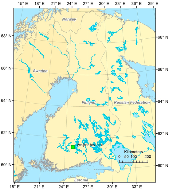
Fig. 1. Location of the study area.
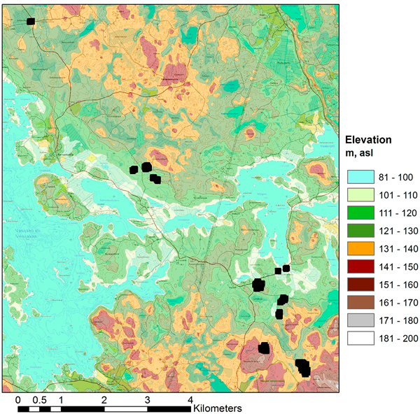
Fig. 2. Layout of the 11 test sites in the study area (topographic map and elevation model © National Land Survey of Finland, 2014).
In the analysis the trees were separated into the following species groups: pine, spruce, larch and broadleaved trees (mainly birch but containing a small portion of non-dominant aspen and grey alder). In the field data, approximately 60% of field plots represent young and middle-aged forests, corresponding roughly to volume classes 100–200 m2 ha–1 and 200–300 m2 ha–1 respectively. From the remaining part, 37 % of the field plots represent volume classes over 300 m2 ha–1 (mature forests) and 3.4% volume class less than 100 m3 ha–1 (mainly advanced seedling stands). The distribution of the measured stand volumes of the field plots is presented in Fig. 3.
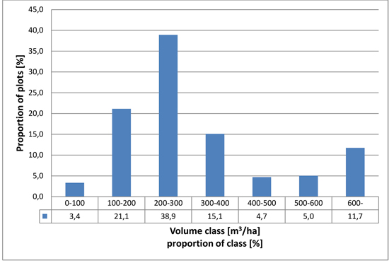
Fig. 3. Distribution of field plots in relation to growing stock volume.
2.2 Aerial imagery
Altogether 11 test sites were captured in 8 UAV flights in 25–26.6.2014 (Table 2, Table 3). The most significant information of the dataset is given in the following, and more details can be found in Nevalainen et al. (2017).
| Table 2. Flight conditions and camera settings during the flights. Median irradiance was taken from Intersil ISL29004 irradiance measurements. Flight height is given from the ground level. | ||||||||
| Area | Date | Time (GPS) | Weather | Solar elevation | Sun azimuth | Median irrad | Exposure (ms) | Flight height (m) |
| v01 | 26.6 | 11:07 to 11:23 | cloudy | 50.91 | 199.22 | 2602 | 10 | 94 |
| v02 | 26.6 | 12:09 to 12:22 | cloudy | 47.38 | 219.63 | 4427 | 12 | 88 |
| v0304 | 25.6 | 10:38 to 10:51 | varying | 51.79 | 188.36 | variable | 6 | 85 |
| v05 | 25.6 | 09:26 to 09:40 | varying | 50.93 | 160.69 | variable | 6 | 86 |
| v0607 | 25.6 | 12:14 to 12:24 | cloudy | 47 | 221.30 | 3773 | 10 | 94 |
| v08 | 26.6 | 09:58 to 10:09 | sunny | 51.84 | 173.41 | 13894 | 10 | 86 |
| v09v10 | 25.6 | 13:51 to 14:12 | cloudy | 37.20 | 249.45 | 2546 | 8 | 84 |
| v11 | 26.6 | 08:49 to 08:58 | varying | 49.1 | 148.44 | 13982 | 10 | 83 |
| Table 3. Results of orientation processing; numbers of GCPs and images, reprojection errors and point density in points m–2. | ||||||
| Block | N GCP | RGB and FPI | RGB | |||
| N images | Reproj. error (pix) | N images | Reproj. error (pix) | Pointcloud points m–2 | ||
| v01 | 7 | 714 | 0.70 | 291 | 0.84 | 484 |
| v02 | 4 | 469 | 0.64 | 176 | 0.73 | 555 |
| v0304 | 9 | 758 | 0.60 | 281 | 0.70 | 711 |
| v05 | 5 | 717 | 0.68 | 292 | 0.89 | 601 |
| v06 | 3 | 193 | 0.91 | 76 | 1.10 | 510 |
| v07 | 4 | 176 | 1.63 | 68 | 2.56 | 524 |
| v08 | 5 | 421 | 0.73 | 178 | 0.99 | 538 |
| v09 | 4 | 280 | 0.57 | 109 | 0.66 | 621 |
| v10 | 3 | 182 | 0.65 | 70 | 0.88 | 484 |
| v11 | 4 | 469 | 0.478 | 469 | 0.478 | 833 |
The UAV platform frame was a Tarot 960 hexacopter with the Pixhawk autopilot equipped with Arducopter 3.15 firmware. Payload capacity of the system is about 3 kg and the flight time is 10–30 min depending on payload, battery, conditions, and flight style. The system setup is shown in Fig. 4.
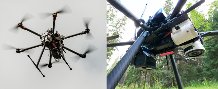
Fig. 4. UAV system (left) based on a Tarot 960 hexacopter and close-up of the sensor configuration (right) (Photographs by Tapio Huttunen).
A hyperspectral camera based on a tuneable Fabry-Pérot interferometer (FPI) (Mäkynen et al. 2011; Saari et al. 2011; Honkavaara et al. 2013) was used to capture the spectral data. The FPI camera captures frame-format hyperspectral images in a time sequential mode; the time lap is 0.075 s between adjacent exposures and 1.8 s during the entire data cube. Because of the time lap each band of the data cube has a slightly different position and orientation, which has to be taken into account in the post-processing phase. The image size was 1024 × 648 pixels and the pixel size was 11 μm. The FPI camera has a focal length of 10.9 mm; the field of view (FOV) is ±18° in the flight direction, ±27° in the cross-flight direction, and ±31° at the format corner. The camera system has an irradiance sensor based on an Intersil ISL29004 photodetector to measure the wideband irradiance during each exposure (Hakala et al. 2013). Spectral settings can be selected according to the requirements. In this study altogether 38 bands were used with a full width of a half maximum (FWHM) of 11–31 nm (Table 4). In order to capture high spatial resolution data, the UAV was also equipped with an ordinary Samsung NX1000 RGB compact digital camera. The camera has a 23.5 × 15.7 mm CMOS sensor with a 20.3 megapixel resolution, and a 16 mm lens.
| Table 4. Spectral settings of the FPI VIS/NIR. L0: central wavelength; FWHM: full width at half maximum. |
| L0 (nm): 507.60, 509.50, 514.50, 520.80, 529.00, 537.40, 545.80, 554.40, 562.70, 574.20, 583.60, 590.40, 598.80, 605.70, 617.50, 630.70, 644.20, 657.20, 670.10, 677.80, 691.10, 698.40, 705.30, 711.10, 717.90, 731.30, 738.50, 751.50, 763.70, 778.50, 794.00, 806.30, 819.70, 833.70, 845.80, 859.10, 872.80, 885.60 |
| FWHM (nm): 11.2, 13.6, 19.4, 21.8, 22.6, 20.7, 22.0, 22.2, 22.1, 21.6, 18.0, 19.8, 22.7, 27.8, 29.3, 29.9, 26.9, 30.3, 28.5, 27.8, 30.7, 28.3, 25.4, 26.6, 27.5, 28.2, 27.4, 27.5, 30.5, 29.5, 25.9, 27.3, 29.9, 28.0, 28.9, 32.0, 30.8, 27.9 |
Flying height from the ground level was 83–94 m providing an average GSD of 8.6 cm for the FPI images and 2.3 cm for the RGB images on the ground level. The flight height was approximately 62–73 m from the tree tops, giving average GSDs of 6.5 cm and 1.8 cm at tree tops for the FPI and RGB data sets, respectively. The flight speed was about 4 m s–1. The FPI image blocks had average forward and side overlaps of 67% and 61%, respectively at the nominal ground level, and 58% and 50%, respectively, at the tree top level. For the RGB blocks, the average forward and side overlaps were 78% and 73%, respectively, at the ground level; at the level of treetops, the average forward and side overlaps were 72% and 65%, respectively.
Imaging conditions were quite windless, but illumination varied a lot. Illumination conditions were cloudy and quite uniform during flights v01, v02, v0607, v0910. Test site v08 was captured under sunny conditions and during flights v0304, v05 and v11 the illumination conditions varied between sunny to cloudy.
2.3 Geometric and radiometric processing of images
2.3.1 Geometric processing
Geometric processing included determination of the orientations of the images and measurement of the 3D point clouds. The Agisoft PhotoScan Professional commercial software (AgiSoft LLC, St. Petersburg, Russia) and Finnish Geospatial Research Institute’s (FGI) in-house software were used for geometric processing. Orientations of the FPI images were determined in integrated processing with the RGB images. Three FPI bands (reference) were included simultaneously in the processing. The numbers of images in the integrated blocks were 176–758 (Table 3). The outputs of the process were the camera calibrations and the image exterior orientations which were transformed to the ETRS-TM35FIN coordinate system using the GCPs in the area. Orientations of the bands of the FPI images that were not included in the orientation processing were determined by matching unoriented bands to the oriented bands using the FGI’s in-house software. Orientations of the RGB dataset were determined also separately without the FPI images, and dense point clouds were then generated using two-times down-sampled RGB images.
Statistics of the geometric processing indicated good accuracy (Table 3). The reprojection errors were mostly 0.6–0.9 pixels; for block v07 the reprojection errors were up to 2.5 pixels, but the data fitted well with the reference airborne laser scanning data that was available from the area. The dense point clouds had point densities of about 500–700 points per m2, and with approximately 5 cm point distance. Point clouds were resampled to a grid CSM with a 5 cm point interval for the study. Height above ground (H) values were calculated for the points by subtracting the ALS-based DTM values from the point Z coordinate values, thus resulting in a canopy height model (CHM).
2.3.2 Radiometric processing
Our objective was to analyse different test areas simultaneously thus it was necessary to scale the radiometric values to a similar scale. The absolute reflectance calibration was the preferred approach. Reflectance reference panels of a size of 1 × 1 m and nominal reflectance of 0.03, 0.09 and 0.50 were installed close to the take-off location in each study site in order to carry out the reflectance transformation using the empirical line method (Smith and Milton 1999). Unfortunately the targets were surrounded by tall trees, thus the illumination conditions in reference targets did not correspond to the illumination conditions on top of the canopy. Because of this they did not provide accurate reflectance calibration by empirical line method. A further challenge was that the illumination conditions were variable during many of the flights, providing large relative differences in radiometric values within the blocks and between different blocks.
Radiometric processing was carried out using the FGI’s in-house software (Honkavaara et al. 2013). Two different radiometric processing options were used. In the first, normalization was not used within or between the blocks, thus the DNs were used directly. Second approach was to transform the DNs to reflectance and use a radiometric block adjustment and inflight irradiance data to normalize the differences within and between the blocks. Area v06 (see Fig. 5b) was selected as the reference area and empirical line-based reflectance calibration was calculated using this area; the disturbance due to surrounding forest vegetation was the least in this area. Radiometric adjustment was calculated within the images of each image block, and then relative correction was calculated between the reference block and each block using the irradiance observations; details of the processing are given by Nevalainen et al. (2017). Examples of uncalibrated and radiometrically calibrated image mosaics are presented in Fig. 5a (changing weather conditions during imaging flight) and Fig. 5b (uniform cloudy weather during imaging flight).
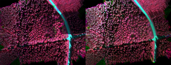
Fig. 5a. Original image mosaic (left) acquired in weather conditions changing from cloudy to clear during imaging flight and radiometrically calibrated mosaic (right).
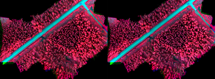
Fig. 5b. Original image mosaic (left) acquired in uniform cloudy weather conditions during imaging flight and radiometrically calibrated mosaic (right).
2.3.3 Mosaic calculation
Hyperspectral orthophoto mosaics were calculated with 10 cm GSD from the FPI images using the FGI’s processing software with the following radiometric processing options: no corrections; absolute calibration and relative normalizations. The RGB mosaics were calculated using the PhotoScan mosaicking module with a 5 cm GSD.
2.4 Extraction of remote sensing features
The remote sensing features were extracted for nine-metre radius circular sample plots, except for textural features where 16 × 16 m windows centred on the sample plots were used. The size was set to correspond to the size of the circular plots.
The following raster features were extracted from calibrated and non-calibrated hyperspectral imagery, true colour (red, green and blue channels) imagery and rasterized point height data:
1. Spectral averages (AVG) of pixel values of channels 1–38 of the hyperspectral imagery and the first principal component calculated using all 38 hyperspectral channels (pixel values with a height above ground less than 2.0 metres were excluded)
2. Standard deviations (STD) of pixel values of data sets as for AVG (pixel values with a height above ground less than 2.0 metres were excluded)
3. Textural features based on co-occurrence matrices of pixel values of hyperspectral channels 18 (red), 36 (near infrared); first band of the principal components images; R, G & B channels of the true colour imagery & H (Haralick et al. 1973; Haralick 1979)
a. Sum Average (SA)
b. Entropy (ENT)
c. Difference Entropy (DE)
d. Sum Entropy (SE)
e. Variance (VAR):
f. Difference Variance (DV)
g. Sum Variance (SV)
h. Angular Second Moment (ASM, also called Uniformity)
i. Inverse Difference Moment (IDM, also called Homogeneity)
j. Contrast (CON)
k. Correlation (COR)
The following features were extracted from photogrammetric (XYZ format) 3D point data (Næsset 2004; Packalén and Maltamo 2006, 2008):
1. Average value of H of vegetation points [m] (HAVG)
2. Standard deviation of H of vegetation points [m] (HSTD)
3. H where percentages of vegetation points (0%, 5%, 10%, 15%, …, 90%, 95%, 100%) were accumulated [m] (e.g. H0, H05,...,H95, H100)
4. Coefficient of variation of H of vegetation points [%] (HCV)
5. Proportion of vegetation points [%] (VEG)
6. Canopy densities corresponding to the proportions points above fraction no. 0, 1, …, 9 to a total number of points (D0, D1, …, D9)
7. Proportion of vegetation points having H greater or equal to corresponding percentile of H (i.e. P20 is the proportion of points having H> = H20) (%) *
8. Ratio of the number of vegetation points to the number of ground points
9. Proportion of ground points (%), where:
H = height above ground
vegetation point = point with H > = 2 m
ground point = other than vegetation point
* the range of H was divided into 10 fractions (0, 1, 2,…, 9) of equal distance
2.5 Feature selection and estimation of forest variables
The k-nearest neighbour (k-nn) method was used for the estimation of the forest variables. The estimated stand variables were total volume of growing stock (volume), the volumes of Scots pine (vol.pine), Norway spruce (vol.spruce), Siberian larch (vol.larch) and broadleaved species (vol.broadleaved), mean diameter (d) and mean height (h). Different values of k were tested in the estimation procedure. In the k-nn estimation (Kilkki and Päivinen 1987; Muinonen and Tokola 1990; Tomppo 1991), the Euclidean distances between the sample plots were calculated in the n-dimensional feature space, where n stands for the number of remote sensing features used. The stand variable estimates for the sample plots were calculated as weighted averages of the stand variables of the k-nearest neighbours (Eq. 1). Weighting by inverse squared Euclidean distance in the feature space was applied (Eq. 2) for diminishing the bias of the estimates (Altman 1992). Without weighting, the k-nn method often causes undesirable averaging in the estimates, especially at the high end of the stand volume distribution, where the reference data is typically sparse.

where:
![]() = estimate for variable y
= estimate for variable y
![]() = measured value of variable y in the ith nearest neighbour plot
= measured value of variable y in the ith nearest neighbour plot

where:
di = Euclidean distance (in the feature space) to the ith nearest neighbour plot
k = number of nearest neighbours
g = parameter for adjusting the progression of weight with increasing distance*
* g = 0: equal weight for all distances; g = 1: weight inverse of distance; g = 2: weight inverse of squared distance, etc.
The accuracy of the estimates was calculated via leave-one-out cross-validation by comparing the estimated forest variable values with the measured values (ground truth) of the field plots. In the cross-validation all circular plots within same experimental plot were excluded from the nearest neighbours. The accuracy of the estimates was measured in terms of the relative root mean square error (RMSE) (Eq. 3) and relative bias (Eq. 4).


where:
![]() = measured value of variable y on plot i
= measured value of variable y on plot i
![]() = estimated value of variable y on plot i
= estimated value of variable y on plot i
![]() = mean of the observed values
= mean of the observed values
n = number of plots.
The remote sensing datasets encompassed a total of 144 aerial photograph features, 11 features from rasterised canopy height data and 35 3D point features. All aerial image and point features were scaled to a standard deviation of 1. This was done because the original features had very diverse scales of variation. Without scaling, variables with wide variation would have had greater weight in the estimation, regardless of their capability for estimating the forest variables.
Feature selection was carried out with two sets of features. One including features extracted from calibrated, the other from non-calibrated, hyperspectral imagery. From here on these are referred to as calibrated feature set and non-calibrated feature set.
The extracted feature set was large, presenting a high-dimensional feature space for the k-nn estimation. In order to avoid the problems of the high-dimensional feature space, i.e. the “curse of dimensionality”, which is inclined to complicate the nearest neighbour search (Beyer et al. 1999; Hinneburg et al. 2000), the dimensionality of the data was reduced by selecting a subset of features with the aim of good discrimination ability. The selection of the features was performed with a genetic algorithm (GA) -based approach, implemented in the R language by means of the Genalg package (Willighagen and Ballings 2015; R Development Core Team 2016). This approach searches for the subset of predictor variables based on criteria defined by the user. Although there is no guarantee of finding the optimal predictor variable subset (Garey and Johnson 1979), and the algorithm does not go through all possible combinations, solutions close to optimal can usually be found in a feasible computational time.
The general GA procedure begins by generating an initial population of strings (chromosomes or genomes), which consist of a random combination of predictor variables (genes). Each chromosome is considered a binary string having values 1 or 0indicating that certain variable is either “selected” in the subset or “not selected”. The strings evolve over a user-defined number of iterations (generations). This evolution includes the following operations: selecting strings for mating by applying a user-defined objective criterion (the more copies in the mating pool, the better), allowing the strings in the mating pool to swap parts (cross over), causing random noise (mutations) in the offspring (children), and passing the resulting strings to the next generation. The process is repeated until a pre-defined criterion is fulfilled or a pre-determined number of iterations have been completed (Broadhurst et al. 1997; Tuominen and Haapanen 2013; Moser et al. 2017).
Here the evaluation function of the genetic algorithm was employed to minimise the RMSEs of k-nn estimates for each variable in leave-one-out cross-validation. The feature selection was carried out for a combined set of forest variables as well as separately for each forest variable. The sets of selected features are referred to as common (for all variables at the time) or individual (for one variable at the time) from here on. In the combined set the individual forest variables were weighted as follows:
• total volume of growing stock: 30%
• volume of pine: 10%
• volume of spruce: 10%
• volume of larch: 10%
• volume of broadleaved trees: 10%
• stand mean height: 20%
• stand mean diameter: 10%
All 298 plots were used in the GA procedure for testing each generation of features.
In the selection procedure, the population consisted of 200 binary chromosomes, and the number of generations was 60. Thirteen feature-selection runs were carried out for all forest variables at one time as well as separately for each variable to find the feature set that returned the best evaluation value. In selecting the feature weights, floating point chromosomes with values in the range of 0–1 were used and the number of generations was set to 60. Otherwise the selection procedure was similar to the feature selection. The values for parameters k and g (Eq. 1 and 2) were selected during the test runs. When selecting common features for all forest variables the number of nearest neighbours was 3 and 5, and g was 2.6 and 2.9 for the calibrated and non-calibrated feature set, respectively. When selecting features individually for each forest variable the number of nearest neighbours varied between 3 and 6 for both feature sets depending on the variable, and g was between 1.5 and 2.6 for the calibrated feature set, and between 0.7 and 3.0 for the non-calibrated feature set.
3 Results
The main estimation results for the tested forest variables are presented in Table 5a (non-calibrated HS-mosaic & common features), Table 5b (non-calibrated HS-mosaic & individual features), Table 5c (calibrated HS-mosaic & common features) and Table 5d (calibrated HS-mosaic & individual features). The Tables 5a–d present relative RMSE and bias of the estimates, as well as the value of k (number of nearest neighbours) and g (weighting factor within k-nn) returned by the GA. Furthermore, the number of features selected by the GA for each variable is listed in the tables specified for each data type: 3D CHM data (n.3D), HS imagery (n.HS), RGB imagery (n.RGB) and total number of selected features (n.feat). The relative RMSEs for the respective combinations are also illustrated in Fig. 6.
| Table 5a. Estimation results, non-calibrated HS-mosaic, common features. | ||||||||
| Variable | k | g | RMSE (%) | Bias (%) | n.3D.feat. | n.HS.feat. | n.RGB.feat. | n.feat. |
| D | 3 | 2.6 | 18.32 | –2.17 | 7 | 9 | 1 | 17 |
| H | 3 | 2.6 | 8.67 | –0.40 | 7 | 9 | 1 | 17 |
| Volume | 3 | 2.6 | 31.47 | –0.59 | 7 | 9 | 1 | 17 |
| vol.pine | 3 | 2.6 | 45.66 | 0.54 | 7 | 9 | 1 | 17 |
| vol.spruce | 3 | 2.6 | 97.58 | 1.18 | 7 | 9 | 1 | 17 |
| vol.larch | 3 | 2.6 | 91.53 | –1.31 | 7 | 9 | 1 | 17 |
| vol.broadleaved | 3 | 2.6 | 63.98 | –7.26 | 7 | 9 | 1 | 17 |
| n.3D.feat. = number of 3D features; n.HS.feat. = number of hyperspectral features; n.RGB.feat. = number of RGB features; n.feat. = total number of selected features. | ||||||||
| Table 5b. Estimation results, non-calibrated HS-mosaic, individual features. | ||||||||
| Variable | k | g | RMSE (%) | Bias (%) | n.3D.feat. | n.HS.feat. | n.RGB.feat. | n.feat. |
| D | 5 | 0.7 | 14.71 | –0.52 | 4 | 11 | 0 | 15 |
| H | 5 | 1.3 | 7.36 | –0.07 | 4 | 5 | 1 | 10 |
| Volume | 5 | 2.9 | 22.65 | 0.00 | 8 | 7 | 1 | 16 |
| vol.pine | 3 | 0.7 | 40.02 | –0.03 | 4 | 5 | 1 | 10 |
| vol.spruce | 6 | 2.0 | 65.06 | 0.02 | 6 | 18 | 1 | 25 |
| vol.larch | 3 | 3.0 | 45.67 | –3.00 | 6 | 11 | 3 | 20 |
| vol.broadleaved | 5 | 2.0 | 44.52 | 0.04 | 5 | 14 | 2 | 21 |
| n.3D.feat. = number of 3D features; n.HS.feat. = number of hyperspectral features; n.RGB.feat. = number of RGB features; n.feat. = total number of selected features. | ||||||||
| Table 5c. Estimation results, calibrated HS-mosaic, common features. | ||||||||
| Variable | k | g | RMSE (%) | Bias (%) | n.3D.feat. | n.HS.feat. | n.RGB.feat. | n.feat. |
| D | 5 | 2.9 | 19.19 | –1.76 | 9 | 6 | 1 | 16 |
| H | 5 | 2.9 | 9.05 | –0.43 | 9 | 6 | 1 | 16 |
| Volume | 5 | 2.9 | 26.93 | –1.60 | 9 | 6 | 1 | 16 |
| vol.pine | 5 | 2.9 | 41.94 | 0.66 | 9 | 6 | 1 | 16 |
| vol.spruce | 5 | 2.9 | 77.52 | –9.68 | 9 | 6 | 1 | 16 |
| vol.larch | 5 | 2.9 | 60.22 | 2.30 | 9 | 6 | 1 | 16 |
| vol.broadleaved | 5 | 2.9 | 81.98 | –7.10 | 9 | 6 | 1 | 16 |
| n.3D.feat. = number of 3D features; n.HS.feat. = number of hyperspectral features; n.RGB.feat. = number of RGB features; n.feat. = total number of selected features. | ||||||||
| Table 5d. Estimation results, calibrated HS-mosaic, individual features. | ||||||||
| Variable | k | g | RMSE (%) | Bias (%) | n.3D.feat. | n.HS.feat. | n.RGB.feat. | n.feat. |
| D | 5 | 2.0 | 15.20 | –1.76 | 4 | 8 | 0 | 12 |
| H | 6 | 1.5 | 7.50 | –0.14 | 6 | 5 | 3 | 14 |
| Volume | 5 | 2.5 | 23.96 | 0.00 | 8 | 4 | 2 | 14 |
| vol.pine | 5 | 2.0 | 34.51 | 0.00 | 11 | 8 | 0 | 19 |
| vol.spruce | 5 | 2.3 | 57.16 | –0.01 | 6 | 7 | 2 | 15 |
| vol.larch | 3 | 2.6 | 51.07 | –0.29 | 5 | 5 | 2 | 12 |
| vol.broadleaved | 4 | 2.1 | 42.00 | –1.38 | 7 | 13 | 2 | 22 |
| n.3D.feat. = number of 3D features; n.HS.feat. = number of hyperspectral features; n.RGB.feat. = number of RGB features; n.feat. = total number of selected features. | ||||||||
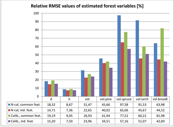
Fig. 6. Relative RMSEs of the estimated forest variables with the tested two calibration options (N-cal = non calibrated; Calib. = calibrated imagery) and feature selection strategies (common features for all variables vs. individual feature set for each variable).
The calibration of the HS mosaic resulted in, to some extent, inconsistent effect in the estimation accuracy when compared to non-calibrated imagery. All estimation results were measured by the relative RMSEs of the tested variables. In the estimation of forest variables related to the size and amount of trees, such as mean diameter, height and total growing stock, the effect of the calibrated HS image mosaic was mostly negligible. The effect of the calibrated HS mosaic was slightly negative in estimating mean height and diameter; the estimation accuracy of diameter decreased 3–5% and height 2–4% (depending on whether RS features were selected for all forest variables at the time or individually for each forest variable). In the estimation of total volume of growing stock, the use of the calibrated mosaic brought about a 14% improvement in the estimation accuracy, when using common features and estimation parameters for all variables, but a 6% decrease, when using features and parameters selected individually for volume estimation.
In the estimation volumes for individual tree species the calibrated mosaic generally performed pronouncedly better than non-calibrated imagery. The estimation accuracy of pine volume was improved 8–14% (with common and individual feature sets, respectively), and spruce volume 12–21%. The results for larch and broadleaved trees were, again, inconclusive. Calibrated imagery gave 34% improvement in the estimation accuracy of larch volume, when using common features and estimation parameters for all variables, but 12% decrease when using features and parameters selected individually for this variable. When estimating the volume of broadleaved trees, calibrated imagery decreased the estimation accuracy by 28%, when using common features and estimation parameters, but improved by 6% when using individually selected features and parameters.
There was a similar but more pronounced difference when comparing estimates based on RS features and estimation parameters common to all variables vs. estimates based on individual features and parameters. Using individually selected features and parameters improved the estimation accuracies of diameter by 20% and 21% (with non-calibrated and calibrated imagery, respectively), height 15% and 17% and total volume of growing stock 28% and 11%, respectively, and whereupon the best total volume estimate was based on features extracted using non-calibrated HS imagery. When estimating volumes per tree species, individually selected features and parameters improved the estimation accuracies (compared to features and estimation parameters common to all variables) for pine 12% and 18% (with non-calibrated and calibrated imagery, respectively), for spruce 33% and 26%, for larch 50% and 15% and for broadleaved trees 30% and 49%. For all tree species except larch, the best estimates were based on features extracted using calibrated HS imagery.
Generally, the accuracy of estimated volume of pine was closest to that of total volume, and it seemed to follow closely the total volume in the estimation results. For other tree species the estimation accuracies were markedly poorer, and had more variation with different feature combinations.
When selecting features and parameters individually for the forest variables, the total number of selected features varied from 10 to 25 and the value of k between 3 and 6. For all forest variables, both 3D features and HS features were highly represented in the selected ones, and their proportion together was approx. 80–100% of the selected features. Features from RGB imagery had low weight in the estimation, and the number of selected RGB features was 0–3. Generally, 3D features were most highly represented in the estimation of height, total volume and also volume of pine. Otherwise, in the estimation of volumes per tree species, HS features were in the majority among the selected ones, as well as in the estimation of diameter. The value of k returned by the GA was in most cases between 4 and 6, but in the estimation of volume of larch k was 3 (as well as for pine volume, in the case of non-calibrated HS mosaic).
When using a common set of features for all forest variables, in total 16–17 features were selected; 3D features were in the majority in the case of calibrated HS mosaic (9/16 of the selected features), whereas HS features were in the majority in the case of non-calibrated HS imagery (9/17 of the selected features); in both cases, only one RGB feature was selected.
Since the GA did not seem to be able to achieve a solution with a common set of features, which would result in good estimation accuracy for both variables related to tree dimension/total volume and volumes per tree species, common feature selection aiming at good tree species recognition that weighted only volumes per main tree species were also tested: pine, spruce and broadleaved trees by 30%, 30% and 40 %, respectively. Only calibrated imagery was used in extracting HS features. This solution was markedly better in the estimation of volumes per tree species than other feature sets common to all forest variables (presented in Tables 5a and 5c). The estimation accuracies (measured by relative RMSEs) were somewhere in the middle between common features sets for all forest variables and individual features for all variables. However, especially the accuracy of the volume of pine was close to that of the individually selected feature set (results presented in Table 6).
| Table 6. Estimation results, calibrated HS-mosaic, features optimized for tree species volumes. | ||||||||
| Variable | k | g | RMSE (%) | Bias (%) | n.3D.feat. | n.HS.feat. | n.RGB.feat. | n.feat. |
| vol.pine | 5 | 3 | 40.63 | –0.43 | 9 | 12 | 3 | 24 |
| vol.spruce | 5 | 3 | 75.78 | –1.56 | 9 | 12 | 3 | 24 |
| vol.broadleaved | 5 | 3 | 50.05 | –0.48 | 9 | 12 | 3 | 24 |
| n.3D.feat. = number of 3D features; n.HS.feat. = number of hyperspectral features; n.RGB.feat. = number of RGB features; n.feat. = total number of selected features. | ||||||||
4 Discussion
The general accuracy of the forest variable estimates in this study was high, when compared to estimates based on ALS and aerial CIR imagery or aerial imagery and photogrammetric 3D data in similar forest conditions. The lowest relative RMSE values for diameter, height and total volume were 14.7%, 7.4% and 22.7% and they were obtained by using individual predictor features for each estimated forest variable. Generally, for research purposes, such as in this case, it is worthwhile to test features tailored to each forest variable individually, whereas in practical forest inventory applications it is typical to use a common feature set for all variables, since the number of inventory variables is often high, and it would not be feasible to have separate features for them.
For comparison, results by, e.g. Järnstedt et al. (2012), who used ALS data with significantly higher point density than typically applied in operational ALS-based forest inventory (approx. 10 pulses m–2), had still significantly larger RMSE values for diameter, height and total volume than presented in this study: 25.3%, 18.6% and 31.3%, respectively. Results by Tuominen et al. (2015) utilizing UAV-borne CIR camera imagery and photogrammetric CSM were also markedly poorer in estimating all tested forest variables; their best estimate for diameter had an RMSE value of 18.4%, height 14.4%, total volume 25.5% and volumes for pine spruce and broadleaved trees 70.9%, 70.7% and 72.8%, respectively. One factor worth noting is that this study, as well as Järnstedt et al. (2012), had extensive field reference data that can be considered well representative for the study area, which makes it possible to have an adequate number of potential reference plots required by the nearest neighbour estimators used in these studies. Instead, field reference data used by Tuominen et al. (2015) was limited in number, which tends to impair the accuracy of nearest neighbour estimates. Puliti et al. (2015) have used UAV-borne CIR camera imagery and photogrammetric 3D data in Norwegian forest areas applying a roughly similar spatial resolution as in this study. Their estimation results are also quite similar to this study, with the exception that Puliti et al. tested also dominant height (which typically correlates highly with 3D canopy models) resulting in very high estimation accuracy with a relative RMSE value of 3.5%. The results may not be fully comparable since the distribution of measured heights and volumes (max–min) in the field data of Puliti et al. was significantly narrower than in this study. When using photogrammetric 3D data in temperate Central European forest conditions, Ullah et al. (2015) have achieved relative RMSEs of 30% for total volume with k-nn estimator (Ullah et al. did not test volume estimation per tree species). Stepper et al. (2016) have reported relative RMSEs of 15.1%, 10.1%, and 35.3% respectively for diameter and height and volume for the spruce-dominated forest, and 15.9%, 9.7%, and 32.1% for the beech-dominated forest, respectively (Stepper et al. have used diameter and height of 100 largest trees ha–1, i.e. dominant diameter and height instead). The distribution and mean of the volume in the field data used by Stepper et al. (2016) was remarkably similar as in this study. Also the mean volume used by Ullah et al. (2015) was in the same magnitude as in this study.
Thus, based on the estimation results of the forest height and volume, it can be assessed that the photogrammetric 3D data used in this study was of remarkably high quality. The contributing factors here presumably are high spatial resolution and sufficient stereo overlap of the original imagery, even despite the fact that the imaging conditions were not optimal because of the challenging illumination conditions due to the changing cloudiness during the imaging flights.
As noted in the results, the calibration of the hyperspectral imagery had practically very little effect on the estimation accuracy of diameter, height and total volume of growing stock, whereas in estimating the volumes of individual tree species, the image calibration had clearly an improving effect on the results in most cases. As expected, the calibrated imagery resulted in higher accuracy for tree species other than larch, for which the effect was contrary to expectations. This, however, may not necessarily indicate any problem in the image calibration, but instead it may be caused by the composition of the field material. Larch formed a significant portion of the total growing stock in relatively few plots, but a number of plots in the high end of the volume distribution were dominated by larch, as indicated by Table 1, where the maximum larch volume was close to maximal total volume. On the other hand, the average volume of larch in the total field data was quite low. Because the volume distribution of the individual tree species was quite different, it is highly likely that 3D features alone were sufficient in predicting volumes of certain species such as larch. If the volume distributions of the tested tree species had been more alike, then the HS features in general would probably have had more weight in their estimation, and the effect of calibration would also have been more evident.
The hyperspectral dataset used in this study was challenging, which might have reduced the achieved accuracy. Conditions during the data capture were typical for the northern climate zone during summer with variable cloudiness and rain. Such conditions are challenging in the case of passive remote sensing because they cause variable image characteristics. As the UAVs are typically operated at low altitudes, and often below cloud cover, it is expected that clouds will cause challenges in many operational applications. Furthermore, the data capture was carried out in deep forest where it was not possible to utilize in-situ reflectance panels in most of the areas. Compensation of the radiometric non-uniformities from the images is necessary in order to normalize the data. The frequently used methods based on reflectance panels or radiative transfer modelling (Zarco-Tejada et al. 2012; Büttner and Röser 2014; Lucieer et al. 2014; Suomalainen et al. 2014) are not suitable in such conditions. The novel radiometric processing approach based on radiometric block adjustment and on-board irradiance measurements (Hakala et al. 2013; Honkavaara et al. 2013) compensated efficiently the differences between the images within flights and between different flights and mostly improved results in variables that were related to tree species. Future studies should improve the methods for radiometric calibration and examine the requirements for radiometric correction.
Our results showed that UAV-based photogrammetry and hyperspectral imaging is a promising method for stand variable estimation. The most important advantage is the markedly improved tree species recognition compared to traditional RGB and CIR aerial imagery, but also the estimation accuracy of variables related to growing stock volume and size equals the accuracy of ALS.
Acknowledgments
This work was supported by the Finnish Funding Agency for Technology and Innovation Tekes through the HSI-Stereo project (grant number 2208/31/2013). The authors also wish to thank Prof. Jari Hynynen of Natural Resources Institute Finland for the support in the acquisition of field data for this study.
References
Aasen H., Burkart A., Bolten A., Bareth G. (2015). Generating 3D hyperspectral information with lightweight UAV snapshot cameras for vegetation monitoring: from camera calibration to quality assurance. ISPRS Journal of Photogrammetry and Remote Sensing 108: 245–259. https://doi.org/10.1016/j.isprsjprs.2015.08.002.
Altman N.S. (1992). An introduction to kernel and nearest-neighbor nonparametric regression. The American Statistician 46(3): 175–185. https://doi.org/10.1080/00031305.1992.10475879.
Anderson K., Gaston K.J. (2013). Lightweight unmanned aerial vehicles will revolutionize spatial ecology. Frontiers in Ecology and the Environment 11(3): 138–146. https://doi.org/10.1890/120150.
Axelsson P. (1999). Processing of laser scanner data – algorithms and applications. ISPRS Journal of Photogrammetry and Remote Sensing 54(2–3): 138–147. https://doi.org/10.1016/S0924-2716(99)00008-8.
Axelsson P. (2000). DEM generation from laser scanner data using adaptive TIN models. International Archives of Photogrammetry and Remote Sensing 33: 110–117.
Baltsavias E. (1999). A comparison between photogrammetry and laser scanning. ISPRS Journal of Photogrammetry and Remote Sensing 54(2–3): 83–94. https://doi.org/10.1016/S0924-2716(99)00014-3.
Baltsavias E., Gruen A., Eisenbeiss H., Zhang L., Waser L.T. (2008). High-quality image matching and automated generation of 3D tree models. International Journal of Remote Sensing 29(5): 1243–1259. https://doi.org/10.1080/01431160701736513.
Beyer K., Goldstein J., Ramakrishnan R., Shaft U. (1999). When is “nearest neighbor” meaningful? In: Proceedings of the 7th International Conference on Database Theory (ICDT ’99), January 10, 1999, Jerusalem, Israel. p. 217–235. https://doi.org/10.1007/3-540-49257-7_15.
Bohlin J., Wallerman J., Fransson J.E.S. (2012). Forest variable estimation using photogrammetric matching of digital aerial images in combination with a high-resolution DEM. Scandinavian Journal of Forest Research 27(7): 692–699. https://doi.org/10.1080/02827581.2012.686625.
Broadhurst D., Goodacre R., Jones A., Rowland J.J., Kell D.B. (1997). Genetic algorithms as a method for variable selection in multiple linear regression and partial least squares regression, with applications to pyrolysis mass spectrometry. Analytica Chimica Acta 348(1–3): 71–86. https://doi.org/10.1016/S0003-2670(97)00065-2.
Büttner A., Röser H.-P. (2014). Hyperspectral remote sensing with the UAS “Stuttgarter Adler” – system setup, calibration and first results. Photogrammetrie – Fernerkundung – Geoinformation 2014(4): 265–274. https://doi.org/10.1127/1432-8364/2014/0217.
Colomina I., Molina P. (2014). Unmanned aerial systems for photogrammetry and remote sensing: a review. ISPRS Journal of Photogrammetry and Remote Sensing 92: 79–97. https://doi.org/10.1016/j.isprsjprs.2014.02.013.
Garey M.R., Johnson D.S. (1979). Computers and intractability; a guide to the theory of np-completeness. W.H. Freeman & Co, New York, NY, USA.
Goetz A.F.H. (2009). Three decades of hyperspectral remote sensing of the Earth: a personal view. Remote Sensing of Environment 113(SUPPL. 1): S5–S16. https://doi.org/10.1016/j.rse.2007.12.014.
Gruen A., Li Z. (2002). Automatic DTM generation from Three-Line-Scanner (TLS) images. International Archives of Photogrammetry and Remote Sensing 34: 131–137.
Haala N., Hastedt H., Wolf K., Ressl C., Baltrusch S. (2010). Digital photogrammetric camera evaluation – generation of digital elevation models. Photogrammetrie – Fernerkundung – Geoinformation 2010(2): 99–115. https://doi.org/10.1127/1432-8364/2010/0043.
Hakala T., Honkavaara E., Saari H., Mäkynen J., Kaivosoja J., Pesonen L., Pölönen I. (2013). Spectral imaging from uavs under varying illumination conditions. In: ISPRS – International Archives of the Photogrammetry, Remote Sensing and Spatial Information Sciences, September 4, 2013, Paris. p. 189–194. https://doi.org/10.5194/isprsarchives-XL-1-W2-189-2013.
Haralick R.M. (1979). Statistical and structural approaches to texture. Proceedings of the IEEE 67(5): 786–804. https://doi.org/10.1109/PROC.1979.11328.
Haralick R.M., Shanmugam K., Dinstein I. (1973). Textural features for image classification. IEEE Transactions on Systems, Man, and Cybernetics SMC-3(6): 610–621. https://doi.org/10.1109/TSMC.1973.4309314.
Hinneburg A., Aggarwal C.C., Keim D.A. (2000). What is the nearest neighbor in high dimensional spaces? In: Proceedings of the 26th International Conference on Very Large Data Bases, September 10, 2000, San Francisco, CA, USA. p. 506–515.
Honkavaara E., Saari H., Kaivosoja J., Pölönen I., Hakala T., Litkey P., Mäkynen J., Pesonen L. (2013). Processing and assessment of spectrometric, stereoscopic imagery collected using a lightweight uav spectral camera for precision agriculture. Remote Sensing 5(10): 5006–5039. https://doi.org/10.3390/rs5105006.
Hruska R., Mitchell J., Anderson M., Glenn N.F. (2012). Radiometric and geometric analysis of hyperspectral imagery acquired from an unmanned aerial vehicle. Remote Sensing 4(9): 2736–2752. https://doi.org/10.3390/rs4092736.
Hyyppä J., Pyysalo U., Hyyppä H., Samberg A. (2000). Elevation accuracy of laser scanning-derived digital terrain and target models in forest environment. In: Proceedings of EARSeL-SIG-Workshop, June 14, 2000, Dresden. p. 139–147.
Järnstedt J., Pekkarinen A., Tuominen S., Ginzler C., Holopainen M., Viitala R. (2012). Forest variable estimation using a high-resolution digital surface model. ISPRS Journal of Photogrammetry and Remote Sensing 74: 78–84. https://doi.org/10.1016/j.isprsjprs.2012.08.006.
Kilkki P., Päivinen R. (1987). Reference sample plots to combine field measurements and satellite data in forest inventory. Department of Forest Mensuration and Management, University of Helsinki, Research Notes 19. p. 210–215.
Koh L.P., Wich S.A. (2012). Dawn of drone ecology: low-cost autonomous aerial vehicles for conservation. Tropical Conservation Science 5(2): 121–132. https://doi.org/10.1177/194008291200500202.
Lillesand T.M., Kiefer R.W., Chipman J.W. (2004). Remote sensing and image interpretation (5th ed.). John Wiley & Sons Inc., New York, NY, USA. p. 763.
Lisein J., Pierrot-Deseilligny M., Bonnet S., Lejeune P. (2013). A photogrammetric workflow for the creation of a forest canopy height model from small unmanned aerial system imagery. Forests 4(4): 922–944. https://doi.org/10.3390/f4040922.
Lucieer A., Malenovský Z., Veness T., Wallace L. (2014). HyperUAS – imaging spectroscopy from a multirotor unmanned aircraft system. Journal of Field Robotics 31(4): 571–590. https://doi.org/10.1002/rob.21508.
Mäkynen J., Holmlund C., Saari H., Ojala K., Antila T. (2011). Unmanned aerial vehicle (UAV) operated megapixel spectral camera. Proceedings of SPIE 8186: 81860Y. https://doi.org/10.1117/12.897712.
Maltamo M., Malinen J., Packalén P., Suvanto A., Kangas J. (2006). Nonparametric estimation of stem volume using airborne laser scanning, aerial photography, and stand-register data. Canadian Journal of Forest Research 36(2): 426–436. https://doi.org/10.1139/x05-246.
Moser P., Vibrans A.C., McRoberts R.E., Næsset E., Gobakken T., Chirici G., Mura M., Marchetti M. (2017). Methods for variable selection in LiDAR-assisted forest inventories. Forestry 90(1): 112–124. https://doi.org/10.1093/forestry/cpw041.
Muinonen E., Tokola T. (1990). An application of remote sensing for communal forest inventory. In: Proceedings from SNS/IUFRO Workshop, 1990, Umeå. p. 35–42.
Næsset E. (2002). Predicting forest stand characteristics with airborne scanning laser using a practical two-stage procedure and field data. Remote Sensing of Environment 80(1): 88–99. https://doi.org/10.1016/S0034-4257(01)00290-5.
Næsset E. (2004). Accuracy of forest inventory using airborne laser scanning: evaluating the first nordic full-scale operational project. Scandinavian Journal of Forest Research 19(6): 554–557. https://doi.org/10.1080/02827580410019544.
Nevalainen O., Honkavaara E., Tuominen S., Viljanen N., Hakala T., Yu X., Hyyppä J., Saari H., Pölönen I., Imai N., Tommaselli A. (2017). Individual tree detection and classification with UAV-based photogrammetric point clouds and hyperspectral imaging. Remote Sensing 9(3): 185. https://doi.org/10.3390/rs9030185.
Packalén P., Maltamo M. (2006). Predicting the plot volume by tree species using airborne laser scanning and aerial photographs. Forest Science 52(6): 611–622.
Packalén P., Maltamo M. (2007). The k-MSN method for the prediction of species-specific stand attributes using airborne laser scanning and aerial photographs. Remote Sensing of Environment 109(3): 328–341. https://doi.org/10.1016/j.rse.2007.01.005.
Packalén P., Maltamo M. (2008). Estimation of species-specific diameter distributions using airborne laser scanning and aerial photographs. Canadian Journal of Forest Research 38(7): 1750–1760. https://doi.org/10.1139/X08-037.
Puliti S., Ørka H.O., Gobakken T., Næsset E. (2015). Inventory of small forest areas using an unmanned aerial system. Remote Sensing 7(8): 9632–9654. https://doi.org/10.3390/rs70809632.
Pyysalo U. (2000). A method to create a three dimensional forest model from laser scanner data. Photogrammetric Journal of Finland 17(1): 34–42.
R Development Core Team. (2016). R: a language and environment for statistical computing. Vienna, Austria. https://www.r-project.org. [Cited 2 March 2017].
Saari H., Pellikka I., Pesonen L., Tuominen S., Heikkilä J., Holmlund C., Mäkynen J., Ojala K., Antila T. (2011). Unmanned Aerial Vehicle (UAV) operated spectral camera system for forest and agriculture applications. In: Proceedings of SPIE, October 6, 2011, Prague. p. 81740H. https://doi.org/10.1117/12.897585.
St-Onge B., Vega C., Fournier R.A., Hu Y. (2008). Mapping canopy height using a combination of digital stereo-photogrammetry and lidar. International Journal of Remote Sensing 29(11): 3343–3364. https://doi.org/10.1080/01431160701469040.
Stepper C., Straub C., Immitzer M., Pretzsch H. (2016). Using canopy heights from digital aerial photogrammetry to enable spatial transfer of forest attribute models: a case study in central Europe. Scandinavian Journal of Forest Research, 1–14. https://doi.org/10.1080/02827581.2016.1261935.
Suomalainen J., Anders N., Iqbal S., Roerink G., Franke J., Wenting P., Hünniger D., Bartholomeus H., Becker R., Kooistra L. (2014). A lightweight hyperspectral mapping system and photogrammetric processing chain for unmanned aerial vehicles. Remote Sensing 6 (11): 11013–11030. https://doi.org/10.3390/rs61111013.
Tomppo E. (1991). Satellite image-based national forest inventory of Finland. International Archives of Photogrammetry and Remote Sensing 28: 419–424.
Törmä M. (2000). Estimation of tree species proportions of forest stands using laser scanning. International Archives of Photogrammetry and Remote Sensing 33(Part B7): 1524–1531.
Tuominen S., Haapanen R. (2011). Comparison of grid-based and segment-based estimation of forest attributes using airborne laser scanning and digital aerial imagery. Remote Sensing 3(5): 945–961. https://doi.org/10.3390/rs3050945.
Tuominen S., Haapanen R. (2013). Estimation of forest biomass by means of genetic algorithm-based optimization of airborne laser scanning and digital aerial photograph features. Silva Fennica 47(1) article 902. https://doi.org/10.14214/sf.902.
Tuominen S., Pitkänen J., Balazs A., Korhonen K.T., Hyvönen P., Muinonen E. (2014). NFI plots as complementary reference data in forest inventory based on airborne laser scanning and aerial photography in Finland. Silva Fennica 48(2) article 983. https://doi.org/10.14214/sf.983.
Tuominen S., Balazs A., Saari H., Pölönen I., Sarkeala J., Viitala R. (2015). Unmanned aerial system imagery and photogrammetric canopy height data in area-based estimation of forest variables. Silva Fennica 49(5) article 1348. https://doi.org/10.14214/sf.1348.
Ullah S., Dees M., Datta P., Adler P., Koch B. (2017) Comparing airborne laser scanning, and image-based point clouds by semi-global matching and enhanced automatic terrain extraction to estimate forest timber volume. Forests 8(6): 215. https://doi.org/10.3390/f8060215.
Vauhkonen J., Tokola T., Packalén P., Maltamo M. (2009). Identification of scandinavian commercial species of individual trees from airborne laser scanning data using alpha shape metrics. Forest Science 55(1): 37–47.
Waser L.T., Ginzler C., Kuechler M., Baltsavias E., Hurni L. (2011). Semi-automatic classification of tree species in different forest ecosystems by spectral and geometric variables derived from Airborne Digital Sensor (ADS40) and RC30 data. Remote Sensing of Environment 115(1): 76–85. https://doi.org/10.1016/j.rse.2010.08.006.
White J.C., Wulder M.A., Vastaranta M., Coops N.C., Pitt D., Woods M. (2013). The utility of image-based point clouds for forest inventory: a comparison with airborne laser scanning. Forests 4(3): 518–536. https://doi.org/10.3390/f4030518.
Willighagen E., Ballings M. (2015). genalg: R based genetic algorithm. https://cran.r-project.org/web/packages/genalg/index.html. [Cited 2 March 2017].
Zarco-Tejada P.J., González-Dugo V., Berni J.A.J. (2012). Fluorescence, temperature and narrow-band indices acquired from a UAV platform for water stress detection using a micro-hyperspectral imager and a thermal camera. Remote Sensing of Environment 117: 322–337. https://doi.org/10.1016/j.rse.2011.10.007.
Total of 58 references.
