Sakari Tuominen  ,
Andras Balazs,
Annika Kangas
,
Andras Balazs,
Annika Kangas
Comparison of photogrammetric canopy models from archived and made-to-order aerial imagery in forest inventory
Tuominen S., Balazs A., Kangas A. (2020). Comparison of photogrammetric canopy models from archived and made-to-order aerial imagery in forest inventory. Silva Fennica vol. 54 no. 5 article id 10291. https://doi.org/10.14214/sf.10291
Highlights
- Two photogrammetric canopy models were tested in forest inventory: one based on archived standard aerial imagery acquired for ortho-mosaic production and another based on stereo-photogrammetrically oriented aerial imaging adjusted for stereo-photogrammetric canopy modelling
- Both data sets were tested in the estimation of forest variables
- Despite the differences in imaging parameters, there was little difference in their performance in predicting the forest inventory variables.
Abstract
In remote sensing-based forest inventories 3D point cloud data, such as acquired from airborne laser scanning, are well suited for estimating the volume of growing stock and stand height, but tree species recognition often requires additional optical imagery. A combination of 3D data and optical imagery can be acquired based on aerial imaging only, by using stereo photogrammetric 3D canopy modeling. The use of aerial imagery is well suited for large-area forest inventories, due to low costs, good area coverage and temporally rapid cycle of data acquisition. Stereo-photogrammetric canopy modeling can also be applied to previously acquired imagery, such as for aerial ortho-mosaic production, assuming that the imagery has sufficient stereo overlap. In this study we compared two stereo-photogrammetric canopy models combined with contemporary satellite imagery in forest inventory. One canopy model was based on standard archived imagery acquired primarily for ortho-mosaic production, and another was based on aerial imagery whose acquisition parameters were better oriented for stereo-photogrammetric canopy modeling, including higher imaging resolution and greater stereo-coverage. Aerial and satellite data were tested in the estimation of growing stock volume, volumes of main tree species, basal area and diameter and height. Despite the better quality of the latter canopy model, the difference of the accuracy of the forest estimates based on the two different data sets was relatively small for most variables (differences in RMSEs were 0–20%, depending on variable). However, the estimates based on stereo-photogrammetrically oriented aerial data retained better the original variation of the forest variables present in the study area.
Keywords
distribution;
prediction;
forest resources;
mapping;
aerial imaging;
digital stereo-photogrammetry
-
Tuominen,
Natural Resources Institute Finland (Luke), Bioeconomy and Environment, P.O. Box 2, FI-00791 Helsinki, Finland
E-mail
sakari.tuominen@luke.fi
- Balazs, Natural Resources Institute Finland (Luke), Bioeconomy and Environment, P.O. Box 2, FI-00791 Helsinki, Finland E-mail andras.balazs@luke.fi
- Kangas, Natural Resources Institute Finland (Luke), Bioeconomy and Environment, P.O. Box 68, FI-80101 Joensuu, Finland E-mail annika.kangas@luke.fi
Received 18 December 2019 Accepted 10 December 2020 Published 15 December 2020
Views 68239
Available at https://doi.org/10.14214/sf.10291 | Download PDF

Supplementary Files
1 Introduction
Multi-source national forest inventory (MSNFI) technique has been used operationally for producing remote sensing-based information of forest resources in the form of thematic maps and forest statistics for various areas since the 1990s in Finland (Tomppo et al. 2008; Mäkisara et al. 2019). The method is based on combining information from satellite imagery, digital map data and field measurements of national forest inventory (NFI) plots (Tomppo et al. 2008). Since the introduction of the method, the availability of satellite imagery has been improved due to new optical earth observation satellites and open access policies adopted by the satellite operators (Barrett et al. 2016; Saarinen et al. 2018). Despite the new open access satellite data from missions such as the Copernicus Sentinel 2, the main drawback of the MSNFI has remained until today: the accuracy of satellite image-based forest estimates is not sufficient at individual stand level (Tomppo et al. 2008; Tuominen et al. 2017a). For this reason, parallel forest inventory systems are maintained for fulfilling the information requirements of forest management (Tuominen et al. 2014; Kangas et al. 2018).
In variables such as the quantity of aboveground forest biomass or (stem) volume of growing stock, it is difficult to achieve any major improvement in the accuracy of remote sensing-based forest estimates using traditional 2-dimensional (2D) image analysis, due to the low correlation between the forest variables and spectral or textural image features (Tuominen et al. 2017a). A significant improvement in the accuracy can be achieved by using 3-dimensional (3D) remote sensing data, e.g., in the form of LiDAR or photogrammetric points clouds.
Although very well suited for estimating local (stand or pixel level) forest variables, the acquisition cycle of airborne laser scanning (ALS) data is not well suited for MSNFI; due to the relatively long acquisition cycle of LiDAR scanning the temporal resolution is low. Moreover, the continuous areas covered by LiDAR scanning each year are not very large, leading to low numbers of NFI plots in each scanning area (Kangas et al. 2018). Regarding the acquisition cycle and area coverage, aerial imaging is better suited for MSNFI; according to the national aerial imaging program in Finland, each part of the country should be covered with intervals of 5 years, providing sufficient temporal resolution for MSNFI. (Maanmittauslaitos 2019a) On the other hand, cloudy weather may prevent obtaining the data within the planned cycle, which is a risk regarding the suitability of photogrammetric data (Kangas et al. 2019). There are also plans for shortening the ALS rotation from 10 to 6 years (Maanmittauslaitos 2019b), which may improve the suitability of ALS data for MSNFI purposes in the future.
The aerial imagery acquired in the national aerial imaging program is mainly aimed at producing RGB and color-infrared ortho-photo mosaics for mapping, survey, forestry and agricultural purposes. Typically, the imaging parameters such as stereo-coverage and spatial resolution have not been adjusted for stereo-photogrammetric canopy modeling. Nevertheless, the stereo coverage of the imagery is sufficient for deriving stereo-photogrammetric 3D point clouds on the basis of the imagery, including archived old images. Although the canopy height models (CHM) based on such imagery appear somewhat crude and contain fewer features when compared visually e.g. to CHM based on ALS, they still have high potential in predicting forest variables such as stem volume and aboveground biomass (Baltsavias et al. 2008; Järnstedt et al. 2012; Pitt et al. 2014). Although the higher precision and detail of the ALS based CHM leads to better accuracy in the estimated of forest variables (Järnstedt et al. 2012), the difference in the accuracy of predicted forest variables between photogrammetric and ALS based CHMs has in many cases been fairly low (Tuominen et al. 2017a; Kangas et al. 2019). On the other hand, in some studies the differences have been remarkable, for instance Kukkonen et al. (2017) reported a difference in RMSE of total volume to be 10.53 percentage units.
Number of different algorithms have been used for generating stereo-photogrammetric point clouds for estimating forest characteristics (Baltsavias et al. 2008; Haala 2014; Stepper et al. 2017; Goodbody et al. 2018; Ullah et al. 2017; Melin et al. 2017). Regardless of the algorithm used, the image resolution, factors related to viewing geometry and stereo-matching parameters have a significant impact on the quality of image-based point clouds (Goodbody et al. 2019).
While there are no universally applicable criteria for an appropriate image resolution for deriving photogrammetric point clouds, improving the image resolution will produce crisper transitions at geometric shapes such as tree canopies, and supposedly improved 3D data product (Leberl et al. 2010).
Increasing the stereo overlap of the imagery provides another means for potential improvement of the 3D data product. From overlapping images, an object can be visible on multiple image pairs, allowing for multi-view matching, which reduces the opportunity for occlusions, and improves geometric accuracy (Leberl et al. 2010; White et al. 2013). The high overlaps also increase the chances for successful matching of tie-points for avoiding gross errors. The high overlaps also reduce the need for dense ground control points and the deformation caused by errors (Kraus 2004; Leberl et al. 2010; Goodbody et al. 2019).
CHMs based on aerial imagery with centimeter class spatial resolution and stereo overlaps of 60–80% would allow high estimation accuracy for forest variables related to the amount of stem growing stock and the size of individual trees, but such data is not economically or operationally feasible in any large area forest inventory. Evidently, it is possible to adjust the parameters of conventional large area aerial imaging towards better suited for applying stereo-photogrammetric 3D modeling, but this will happen at the expense of cost per ha and area coverage. There is no clear-cut solution, what is a feasible trade-off between the cost of aerial imaging when adjusting resolution and stereo-coverage more suited for stereo-photogrammetric 3D modeling and the improvement of forest estimates potentially achieved.
The objective of this study was to examine the performance of two aerial datasets acquired using different imaging resolutions and stereo overlaps in forest inventory. Specifically, the aim was to find out whether the aerial dataset, whose acquisition was based on imaging parameters that were more purpose built for stereo-photogrammetric canopy modelling would result in significant improvement compared to archived aerial imagery in the accuracy of the estimates of growing stock volume, tree species specific volumes and mean stand height and diameter.
2 Materials
2.1 Study area and field data
The study area is located in central Finland in the municipalities of Virrat and Keuruu. The area covers approximately 75 000 ha of a larger test area used in study by (Tuominen et al. 2017a). The geographical, topographical and ecological characteristics of the study are described in detail in (Tuominen et al. 2017a). Map of the study area is presented in Fig. 1.
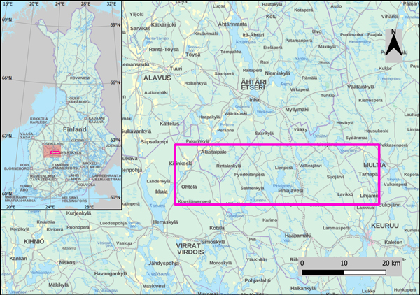
Fig. 1. Map of the study area.
The reference data for this study was allocated in the study area using systematic cluster sampling. The field sample plots were established originally as a part of a larger sample plot network (Tomppo et al. 2016). The field data set consisted of a total of 384 sample plots, of which 312 were located on forestry land. In each of the full clusters, there were eight plots with 250 m spacing in two orthogonal rows, and clusters were placed 4.3 km apart from each other both horizontally and vertically (Tomppo et al. 2016).
The first round of field measurements was carried out in 2013 applying circular 9 m fixed-radius sample plots, from which all trees with diameter (at breast height, DBH) was 4.5 cm or more. Tree species, DBH, tree class, distance and compass bearing from the center point were recorded from all tally trees. Additionally, the mean height and age were measured from the tree of median basal area of each tree species. Additionally, basic stand-level characteristics were measured from each stand intersecting a plot (Tomppo et al. 2016). The plots were re-measured in 2017, excluding the stand-level variables using the same measurement protocols as in 2013. The average values of the field variables measured in 2013 and 2017 were close to each other, but there were differences in the distribution of the field variables measured with 4 year interval, partly due to forest increment and removals, but also due to somewhat differing inclusion of tally trees. The main statistics of field data from years 2013 and 2017 are presented in Table 1. The tree species in the field data are classified as follows: pine, i.e Scots pine (Pinus sylvestris L.), spruce, i.e. Norway spruce (Picea abies (L.) Karst.) and deciduous, i.e. all deciduous tree species (consisting mainly of birches, Betula pendula Roth and B. pubescens Ehrh.). Additionally, the distributions of the volumes of main tree species measured in 2013 and 2017 are presented in Fig. 2.
| Table 1. The main statistics of the field data; mean, median, standard deviation (std) and maximum (max) of the 2013 and 2017 field data sets. | ||||||||
| 2013 | 2017 | |||||||
| Variable | mean | median | std | max | mean | median | std | max |
| Volume, m3 ha–1 | 126.3 | 121.4 | 81.5 | 380.8 | 126.1 | 113.9 | 88.6 | 475.5 |
| Pine volume, m3 ha–1 | 76.4 | 66.2 | 66.3 | 306.6 | 74.9 | 68.0 | 69.1 | 366.4 |
| Spruce volume, m3 ha–1 | 29.4 | 6.4 | 51.6 | 367.8 | 31.4 | 6.3 | 53.5 | 390.0 |
| Deciduous volume, m3 ha–1 | 20.5 | 7.5 | 32.3 | 215.6 | 19.8 | 4.4 | 33.8 | 218.1 |
| DBH, cm | 16.3 | 16.5 | 6.8 | 36.2 | 16.9 | 17.7 | 7.6 | 50.8 |
| Height, m | 13.4 | 14.1 | 5.1 | 27.2 | 13.7 | 14.9 | 5.6 | 25.9 |
| Basal area, m2 ha–1 | 17.3 | 17.4 | 8.7 | 45.0 | 16.4 | 16.3 | 9.3 | 50.6 |
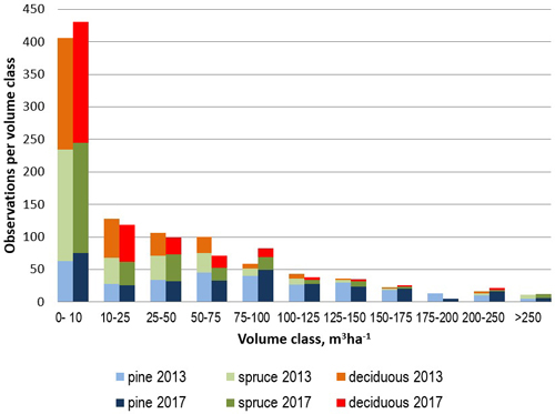
Fig. 2. Distribution of the species-specific growing stock volume classes in the 2013 and 2017 sample plot data sets.
2.2 Remote sensing data
Two sets of remote sensing data corresponding to the dates of the two field measurements were tested in this study. Data set corresponding to year 2013 consisted of aerial imagery acquired in July and August of that year originally with the purpose of aerial ortho-mosaic production for forest management. Imagery was acquired using a Microsoft UltraCam Eagle camera, which is a frame camera. The imaging altitude was 4700 m, and the original imagery had stereo overlap (forward) of 80% and (lateral) 35%. Images contained red (R), green (G), blue (B) and near-infrared (NIR) spectral bands, and they were ortho-rectified to a ground resolution of 30 cm per pixel. Based on the photogrammetric measurements of stereo pair images, a 3D point cloud (canopy surface model, CSM) representing the uppermost canopy layer was calculated using Trimble MATCH-T software. This point cloud covers the study area in the form of an evenly spaced grid with 0.75 m intervals between points (point density approx. 1.8 points m–2). The features extracted from this data are hereafter referred as standard (aerial) data set.
Additionally, Landsat 8 satellite images were used to complement the aerial imagery, since it has been noted that the higher spectral resolution of multispectral satellite imagery provides information not contained by typical color-infrared aerial imagery, and their combination usually lead in to more accurate forest estimates than each of the image data individually. As no suitable Landsat 8 materials were available from summer 2013, a scene acquired on July 23rd 2014 was used for covering the main part of the study area. As that image was partly covered by clouds, another Landsat 8 scene acquired on July 3rd 2015 was used to cover the patches affected by clouds and their shadows. From available Landsat products, atmospherically corrected surface reflectance products were downloaded from USGS EarthExplorer data access portal. The reflectance histograms of the 2015 image bands (bands 1–7) were matched to those of the 2014 image, and the clouded patches of 2014 were filled with the data of 2015.
Aerial imaging-based remote sensing data set corresponding to year 2017 was acquired using Leica DMC III aerial camera which has a push broom sensor. The imaging altitude was same as in 2013 (4700 m), and the stereo overlap was somewhat higher compared to that of 2013: 80% (forward) and 60% (lateral). The average ground sampling distance was 25 cm. Stereo-photogrammetric point cloud was derived from the imagery (using Trimble MATCH-T software) with 25 cm distances between points (point density approx. 16 points m–2). The features extracted from this data are hereafter referred as stereo-oriented (aerial) data set.
Examples of the stereo-photogrammetric point clouds are illustrated in Fig. 3.
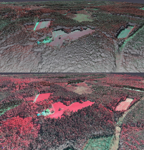
Fig. 3. Oblique view of the stereo-photogrammetric point clouds (points are colored with the spectral values of CIR image bands) based on the standard (top) and stereo-oriented (bottom) aerial data sets. Note the lower point density of the standard data visible in the foreground (there is a new clear-cut in the forefront of the point cloud derived from stereo-oriented image data).
As in standard aerial data set, a contemporary satellite image was used to complement aerial imagery and photogrammetric point cloud. Sentinel 2 image from 30th June 2017 was used to cover most of the test area, but as in Landsat images from 2013the temporally most fitting image scene had cloud gaps, which were covered using another Sentinel image from 17th June 2017.
3 Methods
3.1 Remote sensing features
The stereo-photogrammetric point cloud CSMs derived from the aerial image datasets were converted to canopy height models (CHM) by normalizing the elevation values (Z-coordinates) of the points to terrain level using digital terrain model by National Land Survey of Finland based on airborne laser scanning (Maanmittauslaitos 2020). The canopy height values of the photogrammetric point cloud were also interpolated into a raster format CHMs at spatial resolution and grid spacing similar to the digital aerial images.
Remote sensing features from raster format aerial data were extracted based on 16 × 16 m square windows, whose centers coincided with the centers of the sample plots. The following features were extracted:
1. Averages of pixel values of green, red and near-infrared (NIR) bands.
2. Standard deviations of pixel values of green, red and NIR bands.
3. Textural features based on co-occurrence matrices of pixel values (Haralick et al. 1973; Haralick 1979):
• Angular Second Moment
• Contrast
• Correlation
• Variance
• Inverse Difference Moment
• Sum Average
• Sum Variance
• Sum Entropy
• Entropy
• Difference Variance
• Difference Entropy
• Information Measures of Correlation 1
• Information Measures of Correlation 2
The textural features based on co-occurrence matrices of pixel values were extracted as average values for features calculated in four directions in the extraction window: horizontally (0° angle), vertically (90°), and diagonally (45° and 135°). Lags of 2.7 and 5.7 and 2.5 and 5.0 m were used for standard and stereo-oriented data sets respectively.
From the Landsat and Sentinel satellite imagery, the image features were extracted using single pixels on which the sample plots were located. The following features were extracted:
1. Pixel values of the image bands.
2. Ratios of all possible band combinations (excluding reciprocals).
3. Normalized difference vegetation index (NDVI).
4. Normalized difference vegetation index green (NDVIGreen).
Features from the photogrammetric point clouds were extracted from a circular area of 9 meter radius from each sample plot center. The following point cloud features were extracted (Næsset 2002; Maltamo et al. 2006; Antonarakis et al. 2008):
1. Average, standard deviation and coefficient of variation of height (H) for canopy points.
2. H at which p% of cumulative sum of H of canopy points is achieved; Hp, where p is one of 0, 5, 10, 20, 30, 40, 50, 60, 70, 80, 85, 90, 95 and 100.
3. Percentage of canopy points having H ≥ than corresponding Hp, p is one of 20, 40, 60, 80, 95).
4. Ratio of canopy points to all points.
5. Percentage of canopy points above height limits Hmin + s/10 × (Hmax − Hmin), where s is one of 1–9.*
6. Canopy relief ratio.
7. Skewness and Kurtosis.
8. L-moments (L1, L2, L3, L4) and L-moment skewness and kurtosis.
9. Quadratic mean and cubic mean.
10. Average Absolute Deviation.
11. Median of the absolute deviations from the overall median.
12. Inner Volume and outer Volume.
13. Gap Area.
14. Rumple index.
* The range of H was divided into 10 fractions (0, 1, 2, …, 9), of equal distance, where:
H = return/point height above ground,
canopy point = point with H ≥ 1.3 m,
ground point = other than canopy point.
All features were scaled to have a standard deviation of 1. This was done because the original features had very diverse scales of variation. Without scaling, variables with wide variation would have had greater weight in the estimation regardless of their correlation with the estimated forest attributes (Kaghyan and Sarukhanyan 2012; Nair and Bhagat 2019).
3.2 Estimation and testing of forest variables
The k-nearest neighbor (k-nn) method was used for the estimation of the forest variables (Kilkki and Päivinen 1987; Muinonen and Tokola 1990; Tomppo 1991). The estimated stand variables were mean DBH and mean height, basal area, total volume of growing stock (volume), the volumes of Scots pine, Norway spruce and deciduous species.
The remote sensing datasets encompassed a total of 84 aerial photograph features, 32 features from rasterized canopy height data and 49 3D point features. Additionally, a total of 30 and 69 satellite image features were extracted from Landsat and Sentinel imagery respectively (the numbers differ due to the different number of bands in Landsat 8 and Sentinel-2 images). As the extracted feature set was large, presenting a high-dimensional feature space for the estimation, the dimensionality of the data was reduced by selecting a subset of features with the aim of good discrimination ability. The selection of the features was performed with a genetic algorithm (GA) -based approach, implemented in the R language by means of the Genalg package (Willighagen and Ballings 2015; R Development Core Team 2016). The objective of the genetic algorithm was to minimize the RMSEs of the applied forest variable estimates for each variable in leave-one-out cross-validation.
This approach searches for the subset of predictor variables based on criteria defined by the user. Although there is no guarantee of finding the optimal predictor variable subset (Garey and Johnson 1979), and the algorithm does not go through all possible combinations, solutions close to optimal can usually be found in a feasible computational time.
The general GA procedure begins by generating an initial population of strings (chromosomes or genomes), which consist of a random combination of predictor variables (genes). Each chromosome is considered a binary string having values 1 or 0indicating that certain variable is either `selected’ in the subset or `not selected’. The strings evolve over a user-defined number of iterations (generations). This evolution includes the following operations: selecting strings for mating by applying a user-defined objective criterion (the more copies in the mating pool, the better), allowing the strings in the mating pool to swap parts (cross over), causing random noise (mutations) in the offspring (children), and passing the resulting strings to the next generation. The process is repeated until a pre-defined criterion is fulfilled or a pre-determined number of iterations have been completed (Broadhurst et al. 1997; Tuominen and Haapanen 2013; Moser et al. 2017).
Different values of k were tested in the estimation procedure. In the k-nn estimation, the Euclidean distances between the sample plots were calculated in the feature space defined by the applied remote sensing features. The stand variable estimates for each sample plots were calculated as weighted averages of the stand variables of the k-nearest neighbors (Eq. 1).

where:
![]() = estimate for variable y,
= estimate for variable y,
k = number of nearest neighbors,
![]() = measured value of variable y in the ith nearest neighbor plot.
= measured value of variable y in the ith nearest neighbor plot.
Weighting by inverse squared Euclidean distance in the feature space was applied (Eq. 2) for diminishing the bias of the estimates (Altman 1992). Without weighting, the k-nn method often causes undesirable averaging in the estimates, leading to over- or underestimation in the peripheral areas of forest variable distribution, especially when limited number of reference plots are available.

where:
di = Euclidean distance (in the feature space) to the ith nearest neighbor plot,
g = parameter for adjusting the progression of weight with increasing distance.
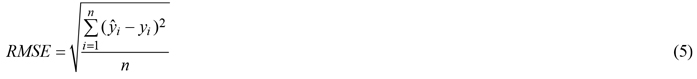
The accuracy of the estimates was calculated via leave-one-out cross-validation by comparing the estimated forest variable values with the measured values (ground truth) of the field plots. In the cross-validation all circular plots within same experimental plot were excluded from the nearest neighbors. The accuracy of the estimates was measured in terms of the relative root mean square error (RMSE) (Eq. 3), relative bias (Eq. 4) and coefficient of determination (R2) between estimated and measured forest variables.


where:
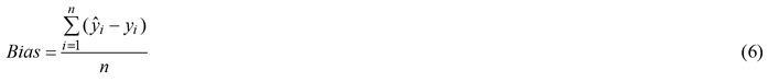
![]() = mean of the observed values,
= mean of the observed values,
n = number of plots.
It is also of interest to assess, how well the distribution of predicted values matches with the distribution of the true values. Especially the predictions in the high and low tails of the distribution are of interest. In this study, the distributions were assessed using an error index defined as:

where p is the number of classes of the distribution considered, ![]() is the true mean volume in the kth class, and
is the true mean volume in the kth class, and ![]() was the mean of predicted volumes in the kth class. This index was calculated for the distribution of total volume and the species-level volume distributions and both datasets.
was the mean of predicted volumes in the kth class. This index was calculated for the distribution of total volume and the species-level volume distributions and both datasets.
4 Results
When comparing the height where 80% of the CHM points of a sample plot were accumulated (H80) to the mean stand height measured from the plot, which typically have high correlation with each other in point cloud data sets, there are practically no differences in the correlation between H80 and mean height in the standard and stereo-oriented data (Fig. 4). The R2 values differ only in the second decimal. In the point cloud data sets from both years there seem to be clear geometric errors in certain sample plots, where the point cloud indicated very low stand height compared to field measurement.
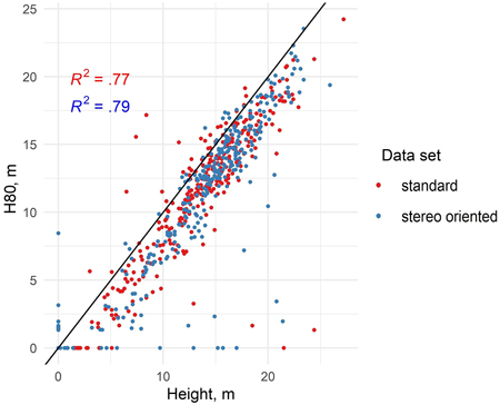
Fig. 4. Scatterplot showing the height at which 80% of canopy points are accumulated (H80) and stand mean height in standard and stereo-oriented data (linear trend line included).
There was little difference in the general estimation accuracies between the standard and stereo-oriented data sets, which can be noted in the scatterplots (Fig. 5) representing the observed values of total volume of growing stock, mean DBH, mean height and basal area and the respective estimated values based on standard and stereo-oriented aerial data. Similar results can be seen from the RMSE values of the estimates, as presented in Table 2 as well. Except for pine and spruce volumes, the estimation accuracy of all forest variables was lower when using stereo-oriented aerial data, which was contrary to expectations. The estimation accuracies for those variables (as measured by RMSE values) were 3–6% lower with stereo-oriented data compared to estimates based on standard data set. However, the accuracy of estimates of the spruce volume were 17% higher and estimates of pine volume 2% higher with stereo-oriented data set.
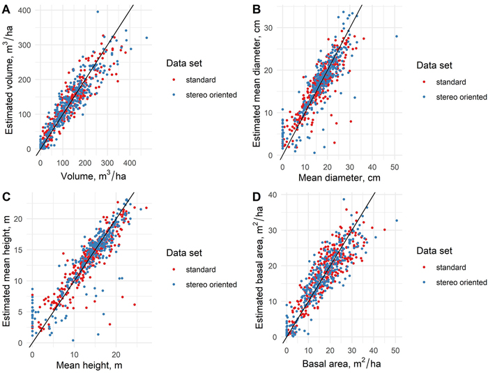
Fig. 5. The scatterplots presenting the measured values of forest variables as well as the values estimated with standard and stereo-oriented data sets.
| Table 2. The accuracy of forest variables (relative RMSE, R2 and relative bias) estimated with standard and stereo-oriented data sets (aerial data only) | ||||||
| RMSE% | R2 | Bias% | ||||
| Standard | Stereo-oriented | Standard | Stereo-oriented | Standard | Stereo-oriented | |
| Volume | 26.50 | 27.44 | 0.85 | 0.86 | 0.10 | –0.41 |
| Pine volume | 53.07 | 52.16 | 0.60 | 0.65 | 1.77 | 5.09 |
| Spruce volume | 136.03 | 112.78 | 0.39 | 0.50 | –0.17 | –10.87 |
| Deciduous volume | 104.94 | 107.75 | 0.39 | 0.43 | –5.74 | –4.62 |
| DBH | 21.93 | 23.16 | 0.71 | 0.75 | –1.16 | –0.08 |
| Height | 18.08 | 19.05 | 0.78 | 0.77 | –0.99 | –0.38 |
| Basal area | 23.98 | 25.46 | 0.76 | 0.79 | 0.56 | 0.08 |
When examining the coefficients of determination (R2) between the estimates based on the standard and stereo-oriented aerial data sets and the respective ground truth values, the R2 were generally slightly higher for variables based on stereo-oriented data set, except for spruce volume, where R2 markedly higher and for mean height estimates where standard data set resulted in slightly higher R2 (Table 2).
When aerial data sets were combined with contemporary satellite imagery, the standard data set combined with Landsat data again resulted in, contrary to expectations, better estimation accuracy for total volume, deciduous volume and basal area compared to stereo-oriented data set (including Sentinel image). However, estimation accuracies for pine and spruce volumes as well as for DBH and height were better when using stereo-oriented aerial data combined with Sentinel data. As with results without satellite data, the only variable showing clear difference in favour of the stereo-oriented data was the volume of spruce, where the estimation accuracy was 20.9% higher than with standard data, as measured by the RMSE. For the volume of pine, the estimation accuracy was 3.3% higher, whereas for the volume of deciduous trees the accuracy was 1.2% lower. The estimation accuracies of DBH and height were 0.4% and 3.3% higher, respectively, with stereo-oriented aerial and Sentinel data. The RMSEs of the estimates based on the combination of aerial and satellite data are presented in Table 3.
| Table 3. The accuracy of forest variables (relative RMSE, R2 and relative bias) estimated with aerial data sets combined with contemporary (Landsat/Sentinel) satellite imagery. | ||||||
| RMSE% | R2 | Bias% | ||||
| Standard | Stereo-oriented | Standard | Stereo-oriented | Standard | Stereo-oriented | |
| Volume | 25.86 | 26.95 | 0.84 | 0.84 | 0.29 | –1.02 |
| Pine volume | 50.71 | 49.02 | 0.66 | 0.73 | 1.77 | 2.91 |
| Spruce volume | 124.96 | 98.81 | 0.50 | 0.66 | –0.59 | –6.27 |
| Deciduous volume | 101.56 | 102.74 | 0.59 | 0.65 | –3.98 | –7.59 |
| DBH | 22.27 | 22.18 | 0.59 | 0.72 | –0.61 | –0.05 |
| Height | 18.49 | 17.88 | 0.76 | 0.78 | –0.95 | –0.63 |
| Basal area | 23.65 | 25.64 | 0.78 | 0.79 | 1.39 | –0.01 |
A more distinct difference between the combinations of aerial and satellite data can be noted when examining the R2 values of the estimates. Again, there was little difference between the two data sets, when estimating total volume, mean height and basal area. However, when estimating species-specific volumes of the main tree species, as well as mean DBH, the coefficient of determination was markedly better when using stereo-oriented aerial and Sentinel data set (see Table 3).
When comparing the distributions of the forest variable estimates based on standard and stereo-oriented aerial data sets with the corresponding field measurements from the sample plots, similar averaging trend was noted for all forest variables. As often typical for k-nn estimates, the classes in the middle of distribution are overestimated, and the classes in the low and especially in the high end of the distribution were underestimated. In the distribution of total growing stock (Fig. 6) volume this trend was less pronounced than in volumes per tree species, and the under-representation is most significant in the highest volume classes of volume estimates based on standard data set. In the estimates based on stereo-oriented data set, the highest volume classes were better represented in relation to the field data. In the total volume distribution, using the same classes as in Fig. 6, the R index was 30.3 for the standard data set and 31.5 for the stereo-oriented data set. Thus, in the total volume the difference was small but to the benefit of standard data set, in the same way as in the RMSE results.
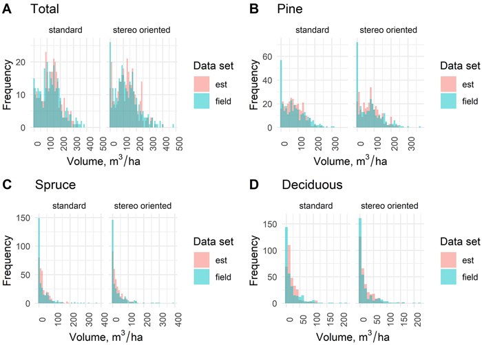
Fig. 6. Distribution of estimated (est) total and species-specific stand volumes based on standard and stereo-oriented data sets and the respective field measurements.
In the distributions of the volumes per tree species (pine, spruce and deciduous) the differences of the measured and estimated (standard vs. stereo-oriented aerial data sets) variables became obvious also in the low end of distribution due to the difficulties in the discrimination of the proportions of tree species with the applied remote sensing data. However, for the volumes of individual tree species, the distributions of the estimated and measured volumes were markedly closer to each other in the stereo-oriented data set for almost all volume classes compared to standard data set. This is confirmed with the R indices, with values 36.45 and 31.47 for pine, 37.47 and 30.01 for spruce and 33.14 and 26.02 for birch in standard and stereo-oriented data sets, respectively. This means that the distributions of the species level results could be improved, even though the distribution of the total volume could not.
In the estimation of stand height (Fig. 7), neither the standard nor the stereo-oriented data set proved clearly better than the other in replicating the height distribution of the measured data from the corresponding year.
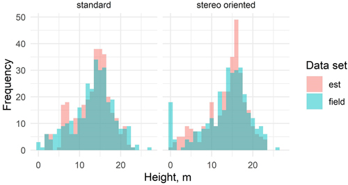
Fig. 7. Distribution of the stand mean height estimates based on standard and stereo-oriented data sets and the respective field measurements.
5 Discussion
The results indicate that customizing the aerial imaging parameters for stereo photogrammetric aerial imaging, while simultaneously aiming at retaining the capability for covering large areas did not bring any marked improvement in the accuracy of the predictions of the forest variables. When examining the accuracy of the total growing stock volume estimates and stand height estimates, whose accuracy is typically highly dependent on the 3D point cloud features, there was no significant difference between the two CHMs that would justify the higher acquisition cost of stereo-oriented imagery. Similarly, when examining the distributions of the total volume and height estimates in comparison with the distributions of field observations, neither the standard nor the stereo-oriented data set demonstrated clear superiority in that regard. When considering the raw point cloud features, such as the height where 80% of points have accumulated (H80) which typically has the highest correlation with stand height, the performance of those point cloud features was virtually similar, as shown by the R2 values presented in Fig. 4, despite the higher point density and geometric quality of CHM based on stereo-oriented data set (as illustrated in Fig. 3).
In the estimation of species specific (pine, spruce and deciduous) growing stock volumes there was some improvement in the plot level accuracies when using the stereo-oriented data, especially in distinguishing the proportions of coniferous species. More significant improvement could be noted, when examining the distributions of species-specific volume estimates, where the stereo-oriented data set seemed to retain better the original variation of the field data in the remote sensing-based estimates. The error indices describing the species-level volume distributions also showed improvement.
When using a combination of aerial and satellite data, which would be a feasible option in practical forest inventory, the inclusion of satellite data generally brought moderate improvement to the estimates based on of both standard and stereo-oriented data sets. The inclusion of satellite data seemed to emphasize the difference of the data sets when estimating species-specific volumes. Here the improvement is mainly due to the better spectral and radiometric resolution of the Sentinel 2 satellite imagery compared to the Landsat 8 imagery. This conclusion can be drawn, when examining the list of RS features selected by GA from the standard and stereo-oriented data sets. Among the features extracted from the stereo-oriented data set, the Sentinel 2 satellite features have higher importance than the Landsat features used with the standard data set. On the other hand, the number of selected CHM and aerial image features in the stereo-oriented data set was notably lower than in the standard data set. However, although lower number of features may indicate their lesser weight in the estimation, sometimes it may also indicate better correlation of individual RS features and field measurements, resulting in fewer features needed. A complete list of features selected from the standard and stereo-oriented data sets is presented in the Supplementary file S1.
Earlier studies (Järnstedt et al. 2012; Gobakken et al. 2015; Tuominen et al. 2017a) have shown that even the much higher geometric detail provided by ALS based CHMs do not result in significantly better forest estimates than photogrammetric CHM with the applied point densities. In that respect the results of this study are highly consistent with other studies comparing different point cloud data sources. However, also studies with a clear difference between photogrammetric data and ALS exist (Kukkonen et al. 2017). The reasons for this kind of variation of the results may depend e.g. on the algorithms used for obtaining the photogrammetric data, and the quality of the aerial photos (for example the shadows of the clouds in the photos). It is likely, that the algorithms can be improved in the future, but the problems due to photo quality are not easily diminished.
When comparing photogrammetric data with varying overlap, Puliti et al. (2017) found 80% overlap slightly outperforms 60%, but Bohlin et al. (2012) reported to have detected no improvement from higher overlap. Our results are also well in line with these studies. It thus seems that utilizing the aerial photos taken for normal forest management are good enough, besides being markedly cheaper.Considerably higher plot level estimation accuracies for similar forest variables as tested in this study have been achieved by using considerably lower level aerial imaging altitudes and UAV-based imaging sensors, which allows significantly higher spatial resolution with similar stereo overlaps as applied in this study (i.e. stereo-oriented data) (e.g. Tuominen et al. 2017b). However, in the present technological situation in UAV-technology, covering large forest areas in the context of NFI, such inventory would not be feasible economically or operationally. In the long run, it is however likely that the development in UAV-technology, as well as increased use of automatization and robotics in their operation will allow covering large forest areas cost-efficiently by UAV-based aerial imaging, while simultaneously enabling the acquisition of geometrically highly accurate CHMs based on spatially high imaging accuracy.
6 Conclusions
The results showed no clear difference between the standard and stereo-oriented aerial data sets in the estimation of forest variables. Thus, there was no conclusive evidence of the advantages brought by the adjustment of the aerial imaging parameters for stereo-photogrammetric 3D modelling instead of using standard aerial imaging parameters intended for ortho-photo production. On the other hand, the results demonstrate the potential benefit of standard aerial imagery which could be put into good use by the application of stereo-photogrammetric 3D modelling. Furthermore, using satellite imagery in combination with aerial data improves the estimation accuracy, especially for the proportions of tree species.
References
Altman N.S. (1992). An introduction to kernel and nearest-neighbor nonparametric regression. The American Statistician 46(3): 175–185. https://doi.org/10.1080/00031305.1992.10475879.
Antonarakis A.S., Richards K.S., Brasington J. (2008). Object-based land cover classification using airborne LiDAR. Remote Sensing of Environment 112(6): 2988–2998. https://doi.org/10.1016/j.rse.2008.02.004.
Baltsavias E., Gruen A., Eisenbeiss H., Zhang L., Waser L.T. (2008). High-quality image matching and automated generation of 3D tree models. International Journal of Remote Sensing 29(5): 1243–1259. https://doi.org/10.1080/01431160701736513.
Barrett F., McRoberts R.E., Tomppo E., Cienciala E., Waser L.T. (2016). A questionnaire-based review of the operational use of remotely sensed data by national forest inventories. Remote Sensing of Environment 174: 279–289. https://doi.org/10.1016/j.rse.2015.08.029.
Bohlin J., Wallerman J., Fransson J.E.S. (2012). Forest variable estimation using photogrammetric matching of digital aerial images in combination with a high-resolution DEM. Scandinavian Journal of Forest Research 27(7): 692–699. https://doi.org/10.1080/02827581.2012.686625.
Broadhurst D., Goodacre R., Jones A., Rowland J.J., Kell D.B. (1997). Genetic algorithms as a method for variable selection in multiple linear regression and partial least squares regression, with applications to pyrolysis mass spectrometry. Analytica Chimica Acta 348(1–3): 71–86. https://doi.org/10.1016/S0003-2670(97)00065-2.
Garey M.R., Johnson D.S. (1979). Computers and intractability: a guide to the theory of NP-completeness. W.H. Freeman & Co, New York, NY, USA.
Gobakken T., Bollandsås O.M., Næsset E. (2015). Comparing biophysical forest characteristics estimated from photogrammetric matching of aerial images and airborne laser scanning data. Scandinavian Journal of Forest Research 30(1): 73–86. https://doi.org/10.1080/02827581.2014.961954.
Goodbody T.R.H., Coops N.C., Hermosilla T., Tompalski P., McCartney G., MacLean D.A. (2018). Digital aerial photogrammetry for assessing cumulative spruce budworm defoliation and enhancing forest inventories at a landscape-level. ISPRS Journal of Photogrammetry and Remote Sensing 142:1–11. https://doi.org/10.1016/j.isprsjprs.2018.05.012.
Goodbody T.R.H., Coops N.C., White J.C. (2019). Digital aerial photogrammetry for updating area-based forest inventories: a review of opportunities, challenges, and future directions. Current Forestry Reports 5: 55–75. https://doi.org/10.1007/s40725-019-00087-2.
Haala N. (2014). EuroSDR-project commission 2 “Benchmark on image matching”, final report. Wien, Austria. http://www.eurosdr.net/sites/default/files/uploaded_files/eurosdr_no64_c.pdf. [Cited 10 July 2020].
Haralick R.M. (1979). Statistical and structural approaches to texture. Proceedings of the IEEE 67(5): 786–804. https://doi.org/10.1109/PROC.1979.11328.
Haralick R.M., Shanmugam K., Dinstein I. (1973). Textural features for image classification. IEEE Transactions on Systems, Man, and Cybernetics SMC-3(6): 610–621. https://doi.org/10.1109/TSMC.1973.4309314.
Järnstedt J., Pekkarinen A., Tuominen S., Ginzler C., Holopainen M., Viitala R. (2012). Forest variable estimation using a high-resolution digital surface model. ISPRS Journal of Photogrammetry and Remote Sensing 74: 78–84. https://doi.org/10.1016/j.isprsjprs.2012.08.006.
Kaghyan S., Sarukhanyan H. (2012). Activity recognition using k-nearest neighbor algorithm on smartphone with tri-axial accelerometer. International Journal ”Information Models and Analyses” 1: 146–156.
Kangas A., Astrup R., Breidenbach J., Fridman J., Gobakken T., Korhonen K.T., Maltamo M., Nilsson M., Nord-Larsen T., Næsset E., Olsson H. (2018). Remote sensing and forest inventories in Nordic countries–roadmap for the future. Scandinavian Journal of Forest Research 33(4): 397–412. https://doi.org/10.1080/02827581.2017.1416666.
Kangas A., Haara A., Holopainen M., Holopainen M., Luoma V., Packalen P., Packalen T., Ruotsalainen R., Saarinen N. (2019). Kaukokartoitukseen perustuvan metsävaratiedon hyötyanalyysi. [Utility analysis of remote sensing-based forest resource data]. Natural Resources Institute Finland (Luke), Luonnonvara- ja biotalouden tutkimus 6/2019. 32 p. http://urn.fi/URN:ISBN:978-952-326-707-7.
Kilkki P., Päivinen R. (1987). Reference sample plots to combine field measurements and satellite data in forest inventory. Department of Forest Mensuration and Management, University of Helsinki, Research Notes 19: 210–215.
Kukkonen M., Maltamo M., Packalen P. (2017). Image matching as a data source for forest inventory – comparison of Semi-Global Matching and Next-Generation Automatic Terrain Extraction algorithms in a typical managed boreal forest environment. International Journal of Applied Earth Observation and Geoinformation 60: 11–21. https://doi.org/10.1016/j.jag.2017.03.012.
Leberl F., Irschara A., Pock T., Meixner P., Gruber M., Scholz S., Wiechert A. (2010) Point clouds: LiDAR versus three-dimensional vision. Photogrammetric Engineering & Remote Sensing 76(10): 1123–1134. https://doi.org/10.14358/PERS.76.10.1123.
Maanmittauslaitos. (2019a). Maastotiedon ylläpito. [Updating field information]. https://www.maanmittauslaitos.fi/maastotiedonkeruu. [Cited 11 Oct 2019].
Maanmittauslaitos. (2019b). Laser2020. http://kmtk.paikkatietoalusta.fi/projektit-ja-tyopaketit/laser2020. [Cited 16 May 2019].
Maanmittauslaitos. (2020). Elevation model 2 m. https://www.maanmittauslaitos.fi/en/maps-and-spatial-data/expert-users/product-descriptions/elevation-model-2-m. [Cited 14 Aug 2020].
Mäkisara K., Katila M., Peräsaari J. (2019). The Multi-Source National Forest Inventory of Finland – methods and results 2015. Natural Resources Institute Finland (Luke), Natural Resources and bioeconomy studies 8/2019. http://urn.fi/URN:ISBN:978-952-326-711-4.
Maltamo M., Malinen J., Packalén P., Suvanto A., Kangas J. (2006). Nonparametric estimation of stem volume using airborne laser scanning, aerial photography, and stand-register data. Canadian Journal of Forest Research 36(2): 426–436. https://doi.org/10.1139/x05-246.
Melin M., Korhonen L., Kukkonen M., Packalen P. (2017) Assessing the performance of aerial image point cloud and spectral metrics in predicting boreal forest canopy cover. ISPRS Journal of Photogrammetry and Remote Sensing 129: 77–85. https://doi.org/10.1016/j.isprsjprs.2017.04.018.
Moser P., Vibrans A.C., McRoberts R.E., Næsset E., Gobakken T., Chirici G., Mura M., Marchetti M. (2017). Methods for variable selection in LiDAR-assisted forest inventories. Forestry 90(1): 112–124. https://doi.org/10.1093/forestry/cpw041.
Muinonen E., Tokola T. (1990). An application of remote sensing for communal forest inventory. Proceedings from SNS/IUFRO Workshop, 35–42. Umeå, Sweden. International Union of Forest Research Organizations.
Nair R., Bhagat A. (2019). Feature selection method to improve the accuracy of classification algorithm. International Journal of Innovative Technology and Exploring Engineering (IJITEE) 8: 124–127.
Næsset E. (2002). Predicting forest stand characteristics with airborne scanning laser using a practical two-stage procedure and field data. Remote Sensing of Environment 80(1): 88–99. https://doi.org/10.1016/S0034-4257(01)00290-5.
Pitt D.G., Woods M., Penner M. (2014). A comparison of point clouds derived from stereo imagery and airborne laser scanning for the area-based estimation of forest inventory attributes in boreal Ontario. Canadian Journal of Remote Sensing 40(3): 214–232. https://doi.org/10.1080/07038992.2014.958420.
Puliti S., Gobakken T., Ørka H.O., Næsset E. (2017). Assessing 3D point clouds from aerial photographs for species-specific forest inventories. Scandinavian Journal of Forest Research 32(1): 68–79. https://doi.org/10.1080/02827581.2016.1186727.
R Development Core Team. (2016). R: a language and environment for statistical computing. http://www.r-project.org. [Cited 2 March 2017].
Saarinen N., White J.C., Wulder M.A., Kangas A., Tuominen S., Kankare V., Holopainen M., Hyyppä J., Vastaranta M. (2018). Landsat archive holdings for finland: Opportunities for forest monitoring. Silva Fennica 52(3) article 9986. https://doi.org/10.14214/sf.9986.
Stepper C., Straub C., Immitzer M., Pretzsch H. (2017). Using canopy heights from digital aerial photogrammetry to enable spatial transfer of forest attribute models: a case study in central Europe. Scandinavian Journal of Forest Research 32(8): 748–61. https://doi.org/10.1080/02827581.2016.1261935.
Tomppo E. (1991). Satellite image-based national forest inventory of Finland. International Archives of Photogrammetry and Remote Sensing 28: 419–424.
Tomppo E., Haakana M., Katila M., Peräsaari J. (2008) Multi-source national forest inventory – methods and applications. Managing Forest Ecosystems 18. Springer. 374 p.
Tomppo E., Kuusinen N., Mäkisara K., Katila M., McRoberts R.E. (2017). Effects of field plot configurations on the uncertainties of ALS-assisted forest resource estimates. Scandinavian Journal of Forest Research 32(6): 488–500. https://doi.org/10.1080/02827581.2016.1259425.
Tuominen S., Haapanen R. (2013). Estimation of forest biomass by means of genetic algorithm-based optimization of airborne laser scanning and digital aerial photograph features. Silva Fennica 47(1) article 902. https://doi.org/10.14214/sf.902.
Tuominen S., Pitkänen J., Balazs A., Korhonen K.T., Hyvönen P., Muinonen E. (2014). NFI plots as complementary reference data in forest inventory based on airborne laser scanning and aerial photography in Finland. Silva Fennica 48(2) article 983. https://doi.org/10.14214/sf.983.
Tuominen S., Pitkänen T., Balázs A., Kangas A. (2017a). Improving Finnish Multi-source National Forest Inventory by 3D aerial imaging. Silva Fennica 51(4) article 7743. https://doi.org/10.14214/sf.7743.
Tuominen S., Balazs A., Honkavaara E., Pölönen I., Saari H., Hakala T., Viljanen N. (2017b). Hyperspectral UAV-imagery and photogrammetric canopy height model in estimating forest stand variables. Silva Fennica 51(5) article 7721. https://doi.org/10.14214/sf.7721.
Ullah S., Dees M., Datta P., Adler P., Koch B. (2017). Comparing airborne laser scanning, and image-based point clouds by Semi-Global Matching and enhanced Automatic Terrain Extraction to estimate forest timber volume. Forests 8(6) article 215. https://doi.org/10.3390/f8060215.
White J.C., Wulder M.A., Vastaranta M., Coops N.C., Pitt D., Woods M. (2013). The utility of image-based point clouds for forest inventory: a comparison with airborne laser scanning. Forests 4(3): 518–536. https://doi.org/10.3390/f4030518.
Willighagen E., Ballings M. (2015). genalg: r based genetic algorithm. https://cran.r-project.org/web/packages/genalg/index.html. [Cited 2 Oct 2019].
Total of 45 references.
