Renats Trubins  ,
Ola Sallnäs
,
Ola Sallnäs
Categorical mapping from estimates of continuous forest attributes – classification and accuracy
Trubins R., Sallnäs O. (2014). Categorical mapping from estimates of continuous forest attributes – classification and accuracy. Silva Fennica vol. 48 no. 2 article id 975. https://doi.org/10.14214/sf.975
Highlights
- The paper presents an approach to classification and accuracy assessment of ad-hoc categorical maps based on existing spatial datasets with estimates of continuous forest variables
- Pixel level class membership probabilities are estimated using a Bayesian network model.
Abstract
Spatially explicit data on forest attributes is demanded for various research with landscape perspective. Existing datasets with estimates of continuous forest variables are often used as the basis for producing categorical forest type maps. Normally, this type of maps are used without knowing their accuracy. This paper presents a Bayesian network model for estimating pixel level class membership probabilities of thus derived categorical maps. Class membership probabilities can be used as a post-classification measure of map accuracy and in the process of map classification affecting the assignments of class labels. The method is applied in mapping deciduous dominated forests on the basis of the k-NN Sweden 2005 dataset in a study area in southern Sweden. The results indicate rather low accuracy for deciduous class regardless of the map classification method: 0.48 versus 0.50 in the maps classified without and with the use of the class membership probabilities given equal deciduous area. When probability-based classification is applied, the level of accuracy varies with the assumed map class proportions. Thus, when deciduous class area corresponding to the National Forest Inventory estimate was used, the accuracy of only 0.35 was obtained for the deciduous map class.
Keywords
Sweden;
land cover maps;
forest type maps;
map accuracy assessment;
class membership probability;
Bayesian network;
k-NN estimates
-
Trubins,
Southern Swedish Forest Research Centre, Swedish University of Agricultural Sciences, Box 49, 230 53 Alnarp, Sweden
E-mail
renats.trubins@slu.se
- Sallnäs, Southern Swedish Forest Research Centre, Swedish University of Agricultural Sciences, Box 49, 230 53 Alnarp, Sweden E-mail ola.sallnas@slu.se
Received 31 July 2013 Accepted 11 March 2014 Published 10 April 2014
Views 115759
Available at https://doi.org/10.14214/sf.975 | Download PDF

1 Introduction
The need for landscape perspective in analysis, implementation and evaluation of forest management, and more broadly land-use has been demonstrated by numerous studies, and is now widely recognized (e.g. Andersson et al. 2006; Hansson and Angelstam 1991; Lindbladh et al. 2011). To implement it in practice relevant information on the state of the landscape is needed. In Sweden, the sample-plot based statistical National Forest Inventory (NFI) is carried out in 5-year cycles since the 1920s. From the NFI data, multiple characteristics of wood stock, forest land and forest ecosystems can be inferred for regional and national levels (Ranneby et al. 1987). A more recent undertaking launched in 2003, the National Inventory of Landscapes in Sweden (NILS) has an overall objective of providing national level data for and performing analyses of landscape biodiversity conditions (Ståhl et al. 2011). However, there are problems that require spatially-explicit, wall-to-wall data coverage. For instance, landscape ecological studies often focus on specific landscape elements or patterns. To meet these needs, several land-cover datasets have been produced over the last decades: the Digital Terrain Type Classification of Satellite Data (TTCSD) from the Swedish Space Corporation in 1900–1991 (Mikusinski et al. 2003), wRESEx from the research program Remote Sensing for the Environment (RESE) (Angelstam et al. 2003) and the Swedish Land Cover Map (SMD) and its upscaled version as a part of the EU CORINE program (Hagner and Reese 2007; Lantmäteriet 2005a). Forest attributes such as standing wood volume by species, mean stand height, age and biomass have been mapped using satellite images and NFI data and compiled in k-NN Sweden (k-NN) datasets (Reese et al. 2003; Reese et al. 2002). Various other methods, including aerial photography and increasingly LIDAR, are used in forest inventories to produce spatially explicit data at lower, for example, estate scales; however, those data are private property held by landowners.
Many recent research with a landscape perspective have used k-NN Sweden or SMD or a combination of the two datasets for identifying or mapping patterns constituted of patches of specific forest types Andersson et al. (2012), Mikusiński and Edenius (2006), Lindbladh et al. (2011), Manton et al. (2005) Stighäll et al. (2011). In principle, k-NN Sweden datasets allow for mapping whatever forest type can be defined on the basis of the forest attributes in the dataset, which means, essentially, creating a new categorical map every time. SMD, in contrast, is limited to the forest classes which are present in the dataset: young, deciduous, mixed and coniferous.
The most straight-forward way of producing a categorical map on the basis of a map (or maps) of continuous variables is what we call a “face value” map classification. It is also the most commonly used method (see, for example, Andersson et al. 2012; Lindbladh et al. 2011; Manton et al. 2005; Mikusiński and Edenius 2006; Paltto et al. 2006; Stighäll et al. 2011). The pixels are classified by directly applying the classification rule to the values of the forest variables from the given dataset (e.g. k-NN Sweden). The classification rule is essentially the class definitions. The classification procedure produces no information on the accuracy of the product. Typically, authors refer to the uncertainty of the forest attribute estimates in the original datasets (e.g. Manton et al. 2005) which is not quite the same thing; an accuracy specification must apply to the actual classes in the map. With no idea of the accuracy, the maps might be, as Mac Roberts (2011) put it, “just pretty pictures”. Due to the costs of the procedure, empirical accuracy assessments are not realistic for maps that are ad-hoc i.e. produced to serve a very specific purpose such as an assessment of a particular habitat type in the landscape. It is for this very reason that this type of maps are derived from existing datasets rather than estimated from spectral records. The first objective of our study was to find a way of estimating the uncertainty of categorical forest type maps that can be derived from the k-NN datasets and to thus improve the scientific and practical validity of their applications. However, the problem and the proposed method are not limited to using k-NN estimated data as the basis for mapping. The estimates of the continuous variables might be based on almost any method; the main problem lies in the transformation of the uncertainty from continuous to categorical variables.
We consider map accuracy to be an expression of map units’ classification (un)certainty and address the problem at pixel level. At pixel level, the (un)certainty of classification can be defined as class membership probabilities (Foody et al. 1992). Richards (1996) demonstrated that class membership probabilities (“accuracy” in his usage) can be derived from known classifier performance and marginal map class proportions intended to represent the prior probabilities of the classes. Steel et al. (2003) went further by trying to actually estimate the performance of a k-NN classifier in the course of image classification in order to obtain the membership probabilities in the same manner as suggested by Richards. The differences in the terminology used by the different authors might be confusing. Steel et al. (2003) speak of “probability of correct classification”, Foody et al. (1992) of “a posteriori probability of membership” and Richards (1996) of “posterior probability” or “accuracy”; all these terms stand for the same concept i.e. the probability that a map unit assigned (or would-be assigned) a certain class label actually belongs to that class. In this paper, we use the term “class membership probability”.
Even though in our problem, existing estimates of continuous forest attributes rather than spectral records serve as predictor variables, it is not fundamentally different. We propose a Bayesian network formulation with the same logic as in the studies cited above. Bayesian network properties allow for effective utilization of the relationships between the forest attributes by modifying the prior probabilities associated with any variable in response to the observed values of the related variables. The class membership probabilities estimated using the Bayesian model can serve not only as a classification accuracy measure but also as a basis for the classification itself. Maps can be classified based on pixel class membership probabilities rather than directly on the forest attribute values (“face values”). Thus, the second objective of the study was to explore the possibilities of probability-based classification methods for improved classification of categorical forest type maps based on the k-NN datasets compared to the “face value” method.
In this study we used the k-NN Sweden 2005 dataset to map deciduous dominated forests in an 8 000 km2 large area in southern Sweden. With the help of the presented method, we estimated pixel class membership probabilities, which we then used to assess the accuracy of a “face-value” map classification and to produce two alternative maps through probability-based classifications. We then compared the maps and discussed the implications of the results for the validity of the method.
2 Method
2.1 Bayesian networks
Estimating class membership probabilities for map units from uncertain predictor variables involves reasoning probabilistically about the values of the variables. Multivariate probabilistic problems can be represented with advantage by graphical models. In our treatment, we use Bayesian network (BN) representation, a graphical model whose graph is a directed acyclic graph. Here, we only offer a concise presentation of the basic ideas; there is an extensive literature on the subject (Murphy 2012; Pearl 2009). As a matter of fact, BN represent joint probability distributions by specifying conditional independence assumptions. By conditional independence is meant that the variables are independent given fixed values of parent variables. In graphs, the nodes represent variables of interest and the links represent causal or information relationships between variables. The strength of a dependency between parent and child nodes is expressed by conditional probabilities usually, but not necessarily, stored in a table. Hence BN can be used to represent any probability distribution of the form

where pai are parent variables of variable xi. With respect to the joint probability distribution each node in the graph corresponds to the factor p(xi | pai). Thus, the pairwise-conditional probabilities are all what is needed to specify the full joint distribution.
2.2 Estimating pixel class membership probabilities
Let us denote the forest attributes covered by a spatial dataset as Yi ∈ (Y1,…,Yn) and the estimates of those attributes as Xi ∈ (X1,…,Xn). Suppose that Yi and Xi are random variables and that the lower case letters denote specific realizations of these variables for each mapping unit j ∈ (1,…,m) on the ground and on the map; then the ground truth is
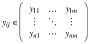
whilst the estimates are
Suppose also that the mapping units in an area of interest need to be classified into a set of disjoint classes C ∈ (c1,…,ck) such that ch ≡ f(y1,…,yn) where ch ∈ C and f is a classification rule corresponding to the class definitions. Then, for any map unit j, the true class is chj ≡ f(y1j,…,ynj). Given the uncertain knowledge of the ground truth, the actual class membership is also uncertain and can be defined as the probability pj(ch) = pj(f(y1j,…,ynj) = ch) so that ![]() . How the pj is computed depends on the actual class definitions and the probability distribution for Y1j,…,Ynj. Hence, in order to obtain class membership probabilities the probability distributions for Y1j,…,Ynj, which specify possible values of the ground truth and their corresponding probabilities, need to be estimated.
. How the pj is computed depends on the actual class definitions and the probability distribution for Y1j,…,Ynj. Hence, in order to obtain class membership probabilities the probability distributions for Y1j,…,Ynj, which specify possible values of the ground truth and their corresponding probabilities, need to be estimated.
Let us first look at YijXij in isolation without considering possible correlations with other variables. The variable Yij could be any of the forest attributes for any pixel j. The value of the estimate Xij can be observed, whilst Yij is hidden. To begin, we can assume that the distribution of Xij, given any yij of the variable Yij is Gaussian. This distribution is the performance of the estimator. The use of normal approximation concerning the distribution of measurements is widely accepted in map classification (Strahler 1980). We can specify the link between the estimated yij and the estimate Xij for any pixel as
![]()
where yij is the mean and σ2 is the variance of the distribution. To employ this model, we must be able to approximate the variance σ2 for any yij.
Having specified the generative model for the data, that is to say the estimator performance, and knowing xij, we can use the prior distribution of the variable P(Yij) = P(Yi) to obtain its posterior distribution P(Yij | xij). Prior probabilities P(Yij) describe our knowledge of how likely different values of the variable Yij are to occur in absence of any information about Xij. The expression takes the familiar form of Bayes theorem,

The left hand side of the expression denotes the posterior distribution of P(Yij) given xij. On the right hand side, P(xij | Yi) is the probability of xij approximated from the generative model (2) given possible values of Yij. Prior probabilities p(Yi) might be known from an independent source or they can be approximated by deriving them from the map itself (Richards 1996). However, in the latter case, the quality of the approximation depends on the unbiasedness of the underlying map estimators.
If correlation exists between the two variables, the posterior probabilities of the variable(s) of interest could be refined by using not only their own estimates but also the estimates of the related variable(s). However, this works only to the degree to which the original estimation errors for the different variables are independent; in this treatment, we assume that they are. This kind of conditional independence assumption is a property of naïve Bayes models which proved to be useful in many fields (Koller and Friedman 2009).
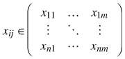
Fig. 1 shows a BN consisting of four variables. Extending the notations used previously, let the nodes Y1j and Y2j represent two forest attributes as random variables, of which only the prior probabilities are known; let X1j and X2j represent the estimates, also as random variables, of Y1j and Y2j respectively. Recall, however, that X1j and X2j can be observed, whilst Y1j and Y2j cannot. According to the graph structure, the full distribution can be factorized as
![]()
In addition to the already familiar terms, this expression contains p(Y2j | Y1j) which specifies the link between the two forest attributes. The conditional probability distribution p(Y2 | Y1) can be either generated, if an independent model of that relationship is available, or estimated from the dataset. The correctness of the latter approximation will, however, depend on the unbiasedness and independence of the estimates. It should be noted that for computational purposes, it is not necessary to actually generate the distributions p(X1j | Y1j) and p(X2j | Y2j) as long as a generative model is specified.
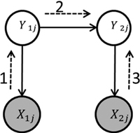
Fig. 1. Bayesian network representation of the joint probability distribution p(X1j, X2j, Y1j, Y2j). Shaded nodes represent the observed variables, the nodes without shading the hidden variables. The solid-line arrows represent the relationships between the variables. The numbered dashed-line arrows show the sequence of message propagation for inferring the posterior distribution of Y2j.
Having thus specified the BN model, the visible variables X1j and X2j can be “clamped” to their observed values x1j and x2j to obtain the conditional p(Y1j | x1j, x2j) and/or p(Y2j | x1j, x2j). Multiple algorithms for message propagation in graphical models are described in literature (e.g. Murphy 2012). A small problem as in our example is not computationally challenging allowing to simply “sum-out” the joint distribution. In Fig. 1, the numbered dashed arrows show the sequence of updating the graph for obtaining p(Y2j | x1j, x2j). Mathematically, propagation against the direction of the links involves Bayes theorem according to the expression (3), whilst propagation along the links involves marginalizing, i.e. summing probabilities of the parental variable over the child variable. In our example, message passing from Y1j to Y2j is realized as
![]()
On the right hand side of the expression is the marginalized conditional distribution of Y2j. The term x1j is included to stress that marginalization was conducted over p(Y1j | x1j). Thus, regardless of the number of variables in the network, we can, by employing expressions (3) and (5), obtain the posterior distributions of the variables of interest for any map unit j. Knowing the class definitions and posterior distributions of the variables, it will not be difficult to compute class probabilities.
3 Application example
In Sweden, deciduous forests are of particular interest for ecological and other research on forestry and land-use embracing landscape perspective. This is reflected by numerous studies focusing, in one or another way, on deciduous forests in a landscape context (e.g. Andersson et al. 2006; Ask 2002; Eriksson et al. 2010; Mikusinski et al. 2003). It means that data on the amount and distribution of deciduous forests in general and of specific deciduous forest types is highly demanded. Some of the needs are met by the NFI; however, often spatially explicit data over entire landscapes are requisite. Therefore, in several studies, k-NN Sweden datasets were used to identify deciduous dominated forest areas.
In this example, we map deciduous dominated forests in Kronoberg County in southern Sweden using the k-NN Sweden 2005 dataset. With the help of the presented method, we estimate class membership probabilities at pixel level, derive the overall measures of accuracy for a map classified at “face-value” and produce two alternative maps by probability-based classification.
3.1 Study area
Kronoberg is located in the hemi boreal zone between the 56th and 57th latitude and has a land area of approximately 849 000 ha (Fig. 2). It is a densely forested region; about 76% of the area is forest land. The forest land ownership pattern is small-scale, dominated by family owners. Norway spruce (Picea abies ( L.) Karst.) accounts for almost half of the standing volume. Scots pine (Pinus sylvestris L.) which is the next most common species makes up about 30% of the standing volume. The deciduous species are mainly represented by birch (Betula spp.) 11%, oak (Quercus spp.) 2.5% and beech (Fagus sylvatica L.) 1% of the standing volume (Nilsson et al. 2008). In the last two decades, the need for increasing the amount of deciduous forests has been emphasized in the environmental debate. Estimated area of deciduous forests, based on the data from the NFI 2001–2005, is 61 000 ha (± 15 000 ha at 95% confidence interval) (NFI 2012).
Fig. 2. Study area Kronoberg County.
3.2 Data
k-NN Sweden are spatially explicit countrywide estimates or forest attributes derived from satellite images and NFI field-plot data produced at the Swedish University of Agricultural Science (Reese et al. 2003; Reese et al. 2002). The datasets owe their names to the estimation algorithm used – k Nearest Neighbor (k-NN). The value of the estimated parameter is calculated as a weighted mean of the k nearest samples in the spectral space. Inverse squared Euclidian distance is used for assigning weights to each of the k samples. In average, some 1250 NFI plots (6-years’ time span) are used in estimation of one satellite scene (Reese et al. 2003). The estimated attributes are standing wood volume by tree species (six individual species and one species group), mean stand age, height and total biomass. The size of pixels is 25*25 meters. As to date, three datasets k-NN Sweden (2000, 2005 and 2010) are available. The accuracy of the estimates in the k-NN Sweden was found to be rather low at a pixel level but improving for averages over larger areas (Reese et al. 2003; Reese et al. 2002). A summary of the reported results regarding pixel level accuracy of k-NN Sweden datasets can be found in Appendix 1.
3.3 Map classes and the probability model
In this example, we defined a set of two classes: deciduous dominated cd and other forests co. Deciduous forest class is defined by the ratio between deciduous and coniferous volume: at least 70% of the total volume has to be deciduous, which roughly corresponds to a ratio of 2.33 between the deciduous and the coniferous volume.
Besides the standing volume which directly enters the forest class definition, we expected that from all the forest attributes in the k-NN dataset, age is most strongly related with species composition. Thus three forest attributes were represented in the model: deciduous volume, coniferous volume and age. We denote the random variables representing the forest attributes as Djy for deciduous volume, Sjy for coniferous volume and Ajy for age for any pixel j ∈ (1,…,m) in the mapping area. Forest class as a dichotomous random variable is denoted by Cjy. The possible outcomes of Cjy are the deciduous class cjd and the other class cjo. The estimates of the forest attributes, also as random variables, are denoted Djx, Sjx and Ajx. Like previously, possible realizations of the random variables are denoted by lower case letters. We use “x” and “y” in superscript to distinguish between the actual forest attributes and their estimates.
Fig. 3 shows a Bayesian network formulation of the problem. The upper part of the graph specifies the dependencies between the forests attributes. Both deciduous Djy and coniferous Sjy volumes correlate with the age Ajy but are assumed to be conditionally independent from each other. Forest class Cjy is a function of the forest attributes Djy and Sjy, which is indicated by the rhomboid shape of the node. The estimates Ajx, Djx and Sjx are conditionally independent from each other and thus only depend on the respective forest attribute variable. The darker fill of the nodes Ajx, Djx and Sjx indicates that these variables can be observed, whilst the nodes without shading represent the hidden variables.
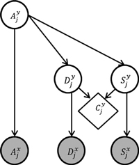
Fig. 3. Bayesian network model for estimating pixels’ class membership probabilities in deciduous forest mapping problem. The variable Djy is deciduous volume, Sjy coniferous volume, Ajy age, and Cjy is forest class. Djx, Sjx and Ajx represent the k-NN estimates of the respective forest attributes. Shaded nodes represent the observed variables, the nodes without shading the hidden variables. The rhomboid shape of the node indicates that Cjy is a deterministic function of Djy and Sjy.
Probability of deciduous forest class p(cjd) for a pixel j is algebraically given by

where dmax is the maximum possible deciduous volume, smax is the maximum coniferous volume and dmin is the minimum deciduous volume. In accordance with the class definition dmin = 2.33sjy. Maximum possible deciduous volume dmax is a constant and so is the maximum coniferous volume defined as smax = 2.33–1dmax. In the computations, we set the maximum deciduous volume equal to the actual highest estimated deciduous volume in the application area.
Since the other class is complementary, the probability of cjo is
![]()
Prior probability distribution for Ajy in the mapping area, and the conditional distributions p(Djy | Ajy) = p(D y | A y) and p(Sjy | Ajy) = p(S y | A y) were approximated using the variable estimates from the k-NN dataset (to represent deciduous and coniferous volumes, volume estimates of corresponding tree species were summed). We treated the variables as discrete and used the empirical distributions derived from the dataset rather than fitting any continuous probability density functions.
With respect to Ajx, Djx and Sjx, i.e. the estimator performance, we assumed Gaussian distributions on grounds discussed earlier. The variances of the distributions were set proportionally to the distributions’ means. In the base case, reported cross-validation RMSE’s were used as coefficients. In addition, sensitivity to the assumed error-level of deciduous volume estimates was tested. Detailed explanation of this point and the parameter values are given in Appendix 1. Since the joint distribution was specified for discrete variables, we used integration over intervals of the probability density function for obtaining the probabilities of ajx, djx and sjx.
For every pixel j, the joint distribution was conditioned on the data, i.e. the observed ajx, djx and sjx. The distributions for the hidden variables were updated according to the graph structure. Since only Djy and Sjy influence the class probabilities directly, Ajy did not need to be updated with the evidence from Djx and Sjx but rather served as a pass for the evidence from Ajx to reach Djy and Sjy. The posterior distributions for Djy and Sjy were used in expression (6) to calculate the posterior probability of cjd.
3.4 Map classification methods
We tested several classification methods. In all cases we used the class definitions specified above.
The first method is what we call “face value classification” (FVC) i.e. a simple classification considering the kNN estimates of the forest variables rather than the computed probabilities (i.e. assuming that djy = djx and sjy = sjx). In FVC, all pixels that fulfill djx ≥ 2.33sjx are classified as deciduous.
Maximum a posteriori classification (MAP) assigns every pixel to the class with the highest class membership probability (Steele 2005). In our case with only two classes it means that all pixels with p(cjd) ≥ 0.5 are labeled as deciduous. However, a preliminary calculation showed that MAP results in only 11 000 ha deciduous (NFI reports 61 000 ha). This clearly showed that a “pure” MAP classification was not suitable in this context and therefore it was excluded from further analyses.
Probability-based classification with predefined class areas maximizes the average membership probabilities for the class as a whole. Maximization is achieved by ranking the pixels according to their probability of class membership and picking the needed number of pixels from the higher end of the range. We tested two different values of deciduous class area. First value was the deciduous area resulting from FVC (27 000 ha, hence MAP27) that allowed for direct comparison of the accuracy values between the two methods. The other value was the NFI estimate of the deciduous area in the region (61 000 ha, hence MAP61). In this case it was of interest to determine the maximum accuracy that could be achieved with such class area.
3.5 Results
In Fig. 4 (a) and (b), the series “Unclassified” show the distribution of all pixels in the application area by the deciduous class membership probability (we will discuss the other series later). Note, that this is pre-classification distribution of pixels. Provided that deciduous dominated forests, by all estimates, constitute less than 10% of the total forest land, naturally, the distribution is dominated by low-probability i.e. very unlikely deciduous pixels. However, the effect is amplified because of the uncertainty associated with the predictor variables. The consistency of the computed probabilities can be roughly tested by calculating the expected map class areas. By summing pixel-level probability values, a figure of approximately 37 000 ha deciduous is obtained which is reasonable number considering the 61 000 ha (±15 000 ha at 95% confidence interval) reported by the NFI (average 2001–2005)(NFI 2012).
Fig. 4 (a) and (b) show the distributions of the pixels labeled as deciduous in each of the three classification methods FVC, MAP27 and MAP61. The distribution in FVC is approximately symmetric with the mode at around 0.50 and ranges from about 0.15 to about 0.85. As mentioned above, the total deciduous area in FVC was 27 000 ha. The distributions of MAP27 and MAP61 are essentially the right hand side of the all-pixels distribution truncated at different points. MAP27 deciduous class encompasses pixels that have class membership probability higher than 0.35 while MAP 61 deciduous class encompasses almost all pixels with the class membership probability above 0.15.
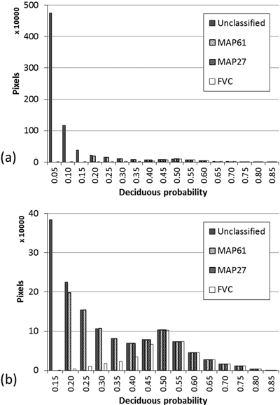
Fig. 4. Distribution of pixels by deciduous class membership probability. Unclassified – all pixels prior to classification; MAP61, MAP27 and FVC – only pixels labeled as deciduous using the respective classificationg method. (a) Full range of values; (b) left-hand side truncated at 0.10.
The average deciduous class membership probability in FVC is 0.48. In MAP27 it is 0.50 corresponding to an improvement of 0.02. The average class membership probability for deciduous pixels in MAP61 is about 0.35.
The sensitivity analysis in which the pixel class membership probabilities were calculated using a different σr value for deciduous (0.75 compared to 1.50 in the base case) resulted in 0.51 for FVC, 0.53 for MAP27 and 0.37 for MAP61. Noteworthy, the differences between the average probability values of the different classifications were preserved and the difference from the base case is small for all methods.
The average class membership probability for the other (“not deciduous”) class in the three maps was: 0.95 for FVC, 0.95 for MAP27 and 0.96 for MAP61. Such high values indicate a very low frequency of misclassification. This outcome is logical considering that the overall class proportion for other forests in the study area is about 90%.
Fig. 5 shows a 4 km2 map fragment with pixels colors scaled according to deciduous class membership probabilities i.e. the unclassified map and the same fragment of the maps classified according to FVC, MAP27 and MAP61. The spatial distribution of pixels with different probability values in the unclassified map exhibits visible regularities. Lower probability-pixels are more frequently found isolated or in small patches while higher probability-pixels occur more often in the core parts of larger contiguous patches. This pattern is plausible considering the fact that edge-pixels are typically prone to estimation errors due to their mixed nature and possible spatial displacement. It is noteworthy that the model produced such spatial pattern even though no spatial relationships at all were considered. In MAP61 there are more deciduous patches and they are more “dense” than in MAP27 and FVC. Between FVC and MAP27 only a small difference can be noticed.
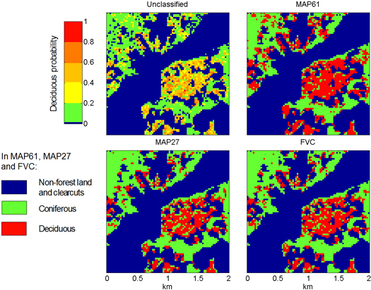
Fig. 5. A fragment of the study area (left bottom corner coordinates x: 1367200, y: 6334550 ; coordinate system RT1990). Unclassified – probability map with no class labels assigned; MAP61, MAP27 and FVC – maps produced using the respective classification method. The bar on the left shows the colors used for different levels of deciduous class membership probabilities in the unclassified map.
Spatial comparison between full FVC and MAP27 (rather than the fragment depicted in Fig. 5) showed that approximately 13% of the deciduous pixels did not match. The substituted pixels in average were “older” than the substituting, 52 years compared to 26 years. This indicates that the model assigned higher probability of deciduous class membership to lower-age pixels, given same ratio of the deciduous and coniferous volumes.
In FVC and MAP 27, the different satellite scenes comprising the map could be clearly distinguished by the amount of deciduous pixels. Also, when displaying the deciduous probabilities prior to any classification, it could be seen that in some scenes the probabilities are mostly low as compared to the other scenes. In contrast, the borders between the satellite scenes are nearly indiscernible in MAP61. Obviously, the low deciduous probabilities and the low number of deciduous pixels in FVC in some scenes are caused by the underestimation of deciduous volume within these scenes in the k-NN dataset (compare the NFI and the FVC estimates). That the magnitude of the bias differs between the scenes is not strange: estimation in kNN Sweden is scene-wise i.e. based on different training data (Reese et al. 2003). For our study, this observation signifies that the probability measures are not completely comparable across the scenes, although the differences between the pixels within individual scenes might be reflected correctly. Nevertheless, the scene level biases in deciduous became less pronounced when larger, and probably more correct, total deciduous area was allocated in MAP61.
In summary, our calculation showed a rather low accuracy of 0.48 for deciduous class in the FVC map. By using a probability-based allocation (MAP27) the accuracy could be improved to 0.50 with the same class area. In general, the user’s accuracy of 0.85 and higher is considered a benchmark for thematic maps. For example, the estimated user’s accuracy of deciduous class in the SMD dataset is 0.69 (Lantmäteriet 2005b). However, considering the notoriously poor accuracy of the k-NN estimates of deciduous volume, the obtained values seem fair. Both in FVC and in MAP27, there were clearly visible differences in the density of deciduous pixels across the satellite scene borders. Increasing the total deciduous class area to the level of the NFI estimate comes at a cost of the class accuracy reduced to 0.35. However, the transitions between satellite scenes smooth out considerably in this case.
4 Discussion
We presented a method for estimating pixel level class membership probabilities when existing remote sensing-based estimates of continuous forest variables are used for map classification. Class membership probabilities allow to produce a probability-based map classification rather than a “face value” classification and to implement a more correct overall class proportion when a reliable independent estimate is available. Measures of overall map classification accuracy, which are necessary to support the user’s confidence in the map, can be readily derived from the pixel level probabilities. In addition, the probability measures on a per pixel base are a valuable supplement to the overall classification accuracy measures and enable a fuller use of the map (Foody et al. 1992). When the intended use of the map is identifying forests with specific characteristics for subsequent field inventory of, for instance, biodiversity values, the class membership probabilities can be considered in selecting the locations to be visited. When, however, the intended use of the map is spatial ecological modeling, the probabilities can be taken into account to adjust the inputs to or the parameters of the models. For example, assume that the quality of a certain habitat type is affected by the amount of a specific forest type within a certain distance. Instead of using the nominal amount of the forest type from the map, we can thus calculate the expected value and use that as the input to the habitat model. Similarly, when studying connectivity, pixels’ probability values can be considered in determining path costs. More simply, only pixels with probabilities above a defined threshold can be selected. If, in contrary, inclusiveness is more important than precision, a larger area than the unbiased estimate suggests can be selected based on probabilities without modifying the class definitions.
The method involves several assumptions. We suggested assuming the variances of the original estimators of the continuous forest variables from empirical relative RMSE’s. RMSE might be a poor basis for approximating the variance; for the kNN data, however, it is presently the only available measure of uncertainty of estimates of continuous forest variables. Once a better estimator of variance is available, it can be used instead. Moreover, the results were rather insensitive to the change of value of the variance parameter for deciduous volume. In the application example, we could not account for biases in the k-NN data due to the lack of relevant assessments. In general, both variance and bias of forest attributes estimated with k-NN technique can vary between scenes due to different sets of reference plots, which we could not account for. The prior probabilities, which also affect the results, can be derived from NFI data rather than from the spatial dataset itself as we did in the example. The same applies to the conditional probabilities when two or more related forest attributes are included in the model. Hence, there are possibilities to use independent data for priors and thus free them from eventual biases the existent spatial dataset. The transparency with respect to the assumptions is an advantage of the method. Furthermore, we would like to note that regardless of the issue of reliability of the model inputs, e.g. RMSE of the k-NN estimates, the method is useful in that it demonstrates the effect of the uncertainty in the underlying continuous forest variables on the accuracy of derived forest type maps.
In summary, the presented method is flexible, transparent and relatively easy to apply. In particular, it can strengthen the validity of inferences made from ad-hoc categorical maps derived from existent remote sensing-based estimates of continuous forest variables, such as kNN Sweden, and encourage their wider and more informed use in ecological and other research with landscape perspective.
References
Andersson K., Angelstam P., Elbakidze M., Axelsson R., Degerman E. (2012). Green infrastructures and intensive forestry: need and opportunity for spatial planning in a Swedish rural–urban gradient. Scandinavian Journal of Forest Research 28(2): 143–165. http://dx.doi.org/10.1080/02827581.2012.723740.
Andersson M., Sallnas O., Carlsson M. (2006). A landscape perspective on differentiated management for production of timber and nature conservation values. Forest Policy and Economics 9(2): 153–161. http://dx.doi.org/10.1016/j.forpol.2005.04.002.
Angelstam P., Mikusinski G., Eriksson J., Jaxgård P., Kellner O., Koffman A., Ranneby B., Roberge J.-M., Rosengren M., Rystedt S., Rönnbäck B.-I., Seibert J. (2003). Gap analysis and planning of habitat networks for the maintenance of boreal forest biodiversity in Sweden: a technical report from the RESE case study in the counties of Dalarna and Gävleborg. County Administrative Board of Dalarna. http://www.lansstyrelsen.se/gavleborg/SiteCollectionDocuments/Sv/miljo-och-klimat/tillstandet-i-miljon/skog/Rapport2003_12_wRESEx.pdf. [Cited 1 March 2013].
Ask P. (2002). Biodiversity and deciduous forest in landscape management. Studies in Southern Sweden. Acta Universitatis Agriculturae Sueciae – Silvestria. ISSN 1401-6230.
Baraldi A., Bruzzone L., Blonda P. (2005). Quality assessment of classification and cluster maps without ground truth knowledge. Geoscience and Remote Sensing, IEEE Transactions on 43(4): 857–873. http://dx.doi.org/10.1109/tgrs.2004.843074.
Eriksson S., Skånes H., Hammer M., Lönn M. (2010). Current distribution of older and deciduous forests as legacies from historical use patterns in a Swedish boreal landscape (1725–2007). Forest Ecology and Management 260(7): 1095–1103. http://dx.doi.org/10.1016/j.foreco.2010.06.018.
Foody G.M., Campbell N.A., Trodd N.M., Wood T.F. (1992). Derivation and applications of probabilistic measures of class membership from the maximum-likelihood classification. Photogrammetric Engineering and Remote Sensing 58(9): 1335–1341.
Hagner O., Reese H. (2007). A method for calibrated maximum likelihood classification of forest types. Remote Sensing of Environment 110(4): 438–444. http://dx.doi.org/10.1016/j.rse.2006.08.017.
Hansson L., Angelstam P. (1991). Landscape ecology as a theoretical basis for nature conservation. Landscape Ecology 5(4): 191–201. http://dx.doi.org/10.1007/bf00141434.
Kim H.-J., Tomppo E. (2006). Model-based prediction error uncertainty estimation for k-nn method. Remote Sensing of Environment 104(3): 257–263. http://dx.doi.org/10.1016/j.rse.2006.04.009.
Koller D., Friedman N. (2009). Probabilistic graphical models: principles and techniques. Massachusetts Institute of Technology, Cambridge–Massachusetts–London. 1233 p.
Lantmäteriet (2005a). Produktspecifikation av svenska CORINE marktäckedata. Dokumentnummer SCMD-0001. Lantmäteriet. http://www.lantmateriet.se/Global/Kartor%20och%20geografisk%20information/Kartor/produktbeskrivningar/SCMDspec.pdf. [Cited 1 March 2013].
Lantmäteriet (2005b). Tematisk noggrannhet i Svenska marktäckedata. Dokumentnummer SCMD-0020. Lantmäteriet. http://www.lantmateriet.se/Global/Kartor%20och%20geografisk%20information/Kartor/produktbeskrivningar/SCMD.pdf. [Cited 1 March 2013].
Lindbladh M., Felton A., Trubins R., Sallnäs O. (2011). A landscape and policy perspective on forest conversion: long-tailed tit (Aegithalos caudatus) and the allocation of deciduous forests in southern Sweden. European Journal of Forest Research: 1–9. http://dx.doi.org/10.1007/s10342-010-0478-9.
Manton M., Angelstam P., Mikusiński G. (2005). Modelling habitat suitability for deciduous forest focal species – a sensitivity analysis using different satellite land cover data. Landscape Ecology 20(7): 827–839. http://dx.doi.org/10.1007/s10980-005-3703-z.
McRoberts R.E. (2011). Satellite image-based maps: scientific inference or pretty pictures? Remote Sensing of Environment 115(2): 715–724. http://dx.doi.org/10.1016/j.rse.2010.10.013.
McRoberts R.E., Tomppo E.O., Finley A.O., Heikkinen J. (2007). Estimating areal means and variances of forest attributes using the k-Nearest Neighbors technique and satellite imagery. Remote Sensing of Environment 111(4): 466–480. http://dx.doi.org/10.1016/j.rse.2007.04.002.
Mikusiński G., Edenius L. (2006). Assessment of spatial functionality of old forest in Sweden as habitat for virtual species. Scandinavian Journal of Forest Research 21(S7): 73–83. http://dx.doi.org/10.1080/14004080500487045.
Mikusinski G., Angelstam P., Sporrong U. (2003). Distribution of deciduous stands in villages located in coniferous forest landscapes in Sweden. Ambio 32(8): 520–526.
Murphy K.P. (2012). Machine learning: a probabilistic perspective. Massachusetts Institute of Technology, Cambridge, Massachusetts. 1065 p.
NFI (2012). Interactive database of National Forest Inventory of Sweden. Swedish University of Agricultural Sciences. http://www-taxwebb.slu.se/Taxwebb/TabellForm/index.html. [Cited 1 March 2013].
Nilsson P., Kempe G., Toet H., Petersson H. (2008). Skogsdata 2008: aktuella uppgifter om de svenska skogarna från Riksskogstaxeringen. SLU, Umeå.
Paltto H., Nordén B., Götmark F., Franc N. (2006). At which spatial and temporal scales does landscape context affect local density of Red Data Book and Indicator species? Biological Conservation 133(4): 442–454. http://dx.doi.org/10.1016/j.biocon.2006.07.006.
Pearl J. (2009). Causality: models, reasoning and inference. Cambridge University Press, New York. 463 p.
Ranneby B., Cruse T., Hagglund B., Jonasson H., Sward J. (1987). Designing a new national forest survey for Sweden. Studia Forestalia Suecica 177: 1–29.
Reese H., Nilsson M., Sandstrom P., Olsson H. (2002). Applications using estimates of forest parameters derived from satellite and forest inventory data. Computers and Electronics in Agriculture 37(1–3): 37–55. http://dx.doi.org/10.1016/S0168-1699(02)00118-7.
Reese H., Nilsson M., Pahlen T.G., Hagner O., Joyce S., Tingelof U., Egberth M., Olsson H. (2003). Countrywide estimates of forest variables using satellite data and field data from the national forest inventory. Ambio 32(8): 542–548. http://dx.doi.org/10.1579/0044-7447-32.8.542.
Richards J.A. (1996). Classifier performance and map accuracy. Remote Sensing of Environment 57(3): 161–166. http://dx.doi.org/10.1016/0034-4257(96)00038-7.
Ståhl G., Allard A., Esseen P.-A., Glimskär A., Ringvall A., Svensson J., Sundquist S., Christensen P., Torell Å., Högström M., Lagerqvist K., Marklund L., Nilsson B., Inghe O. (2011). National Inventory of Landscapes in Sweden (NILS) – scope, design, and experiences from establishing a multiscale biodiversity monitoring system. Environmental Monitoring and Assessment 173(1–4): 579–595. http://dx.doi.org/10.1007/s10661-010-1406-7.
Steele B., Patterson D., Redmond R. (2003). Toward estimation of map accuracy without a probability test sample. Environmental and Ecological Statistics 10(3): 333–356. http://dx.doi.org/10.1023/a:1025111108050.
Steele B.M. (2005). Maximum posterior probability estimators of map accuracy. Remote Sensing of Environment 99(3): 254–270. http://dx.doi.org/10.1016/j.rse.2005.09.001.
Stighäll K., Roberge J.-M., Andersson K., Angelstam P. (2011). Usefulness of biophysical proxy data for modelling habitat of an endangered forest species: the white-backed woodpecker Dendrocopos leucotos. Scandinavian Journal of Forest Research 26(6): 576–585. http://dx.doi.org/10.1080/02827581.2011.599813.
Strahler A.H. (1980). The use of prior probabilities in maximum likelihood classification of remotely sensed data. Remote Sensing of Environment 10(2): 135–163. http://dx.doi.org/10.1016/0034-4257(80)90011-5.
Tokola T., Pitkänen J., Partinen S., Muinonen E. (1996). Point accuracy of a non-parametric method in estimation of forest characteristics with different satellite materials. International Journal of Remote Sensing 17(12): 2333–2351. http://dx.doi.org/10.1080/01431169608948776.
Tomppo E., Olsson H., Ståhl G., Nilsson M., Hagner O., Katila M. (2008). Combining national forest inventory field plots and remote sensing data for forest databases. Remote Sensing of Environment 112(5): 1982–1999. http://dx.doi.org/10.1016/j.rse.2007.03.032.
Total of 35 references
Appendix 1
Analytical derivation of variance estimators for k-NN methods is difficult and not yet widely applied in practice (Tomppo et al. 2008), although some solutions are proposed in the literature, for example (Kim and Tomppo 2006; McRoberts et al. 2007). Typically, the uncertainty of the k-NN predictions is measured by the RMSE, which is estimated empirically. The leave-one-out cross validation method used to estimate RMSE is known to produce unbiased estimates but also to have a large variance (Baraldi et al. 2005).We assumed that variances of Ajx, Sjx and Djx change proportionally to ajy, sjy and djy and used relative RMSE as coefficient. This implies that the variance increases linearly with increasing value of the estimated variable, which is reasonable for medium values of ajy, sjy and djy. However, we imposed bounds on the lowest and the highest values of the variance. Thus, at every instance, the variance was determined as
![]()
where yi ∈ (ajy,sjy,djy); σr is the relative standard deviation approximated by the RMSE for the variable in question; σmin and σmax are the assumed minimum and maximum values of the standard deviation.
Table A1 summarizes the data on RMSE for age and species volume from several Swedish (Reese et al. 2002) and Finnish (Tokola et al. 1996) k-NN applications to forest attribute mapping. Because there were very few published results regarding species-wise volume estimation accuracy from the Swedish projects, the Finnish results were also considered. From the table, it can be seen that the magnitude of errors found in the different studies is similar. For each of the variables, we selected a value from the range of the reported RMSE values. Furthermore, in order to assess the sensitivity of the model to the assumed error-levels, we conducted additional computations using a much lower value for relative standard deviation for deciduous volume.
| Table A1. Pixel level relative RMSE and means for different forest attribute mapping projects using k-NN method. | |||||||
| 1-A | 1-B | 1-C | 1-D | 2-A | 2-B | 2-C | |
| RMSE, age (%) | - | 49 | 57 | 53 | - | - | - |
| Mean age (years) | - | 58.9 | 60.0 | 69.0 | - | - | - |
| RMSE, pine volume (%) | - | 73 | - | - | 147.6 | 131.2 | 121.7 |
| Mean pine volume (m3/ha) | - | - | - | - | - | - | 65.5 |
| RMSE, spruce volume (%) | - | 88 | - | - | 116.0 | 118.2 | 111.7 |
| Mean spruce volume (m3/ha) | - | - | - | - | - | - | 69.2 |
| RMSE, deciduous volume (%) | - | 163.3 | - | - | 157.5 | 206.9 | 148.0 |
| Mean deciduous volume (m3/ha) | - | 18.5 | - | - | - | - | 34.9 |
| RMSE, total volume (%) | 59 | 66 | 58 | 69 | 66.3 | 68.2 | 57.3 |
| Mean total volume (m3/ha) | 120.3 | 165.1 | 187 | 115 | - | - | 80.1 |
| Sources: 1-A Västerbotten, 1-B Gävleborg, 1-C Dalarna and 1-D Älvsbyn projects (Reese et al. 2003; Reese et al. 2002); 2-A and 2-B are two different study areas in Finland; 2-C includes only sample plots located at least 30 m from stand boundary (Tokola et al. 1996). | |||||||
Table A2 shows the assumed values of σr, σmin and σmax. Our assumptions on the lowest and highest values are rather conservative considering that even a very small value of ajy, sjy and djy have considerable probability to be overestimated by 30 or more units and that with increasing value of the variable the standard error can become as high as 150 for age and 250 for volume. For our study, the absolute value of the variance is not as important as the correctly reflected relationship between the variances of Sjx and Djx.
| Table A2. Parameters of the probability distributions for age and volume estimates: relative, minimum and maximum standard deviation. | |||
| σr | σmin | σmax | |
| Age (A) | 50% | 30 years | 150 years |
| Deciduous volume (D) | 150% | 30 m3 | 250 m3 |
| Deciduous volume (D) a) | 75% | 30 m3 | 250 m3 |
| Coniferous volume (C) | 80% | 30 m3 | 250 m3 |
| a) sensitivity analysis | |||
