Juha Lappi  ,
Timo Pukkala
,
Timo Pukkala
Analyzing ingrowth using zero-inflated negative binomial models
Lappi J., Pukkala T. (2020). Analyzing ingrowth using zero-inflated negative binomial models. Silva Fennica vol. 54 no. 4 article id 10370. https://doi.org/10.14214/sf.10370
Highlights
- Models were developed to describe ingrowth in national forest inventory data
- The data were more dispersed than Poisson data and included many zeros
- Fixed-effects models had larger zero-inflation probability and overdispersion parameter than mixed-effect models
- Mixed-effects models had larger likelihood than fixed-effects models but provided biased predictions
- Prediction of right-censored ingrowth may be useful owing to large overdispersion.
Abstract
Ingrowth is an important element of stand dynamics in several silvicultural systems, especially in continuous cover forestry. Earlier predictive models for ingrowth in Finnish forests are few and not based on up-to-date statistical methods. Ingrowth is here defined as the number of trees over 1.3 m entering a plot. This study developed new ingrowth models for Scots pine (Pinus sylvestris L.), Norway spruce (Picea abies (L.) H. Karst.) and birch (Betula pendula Roth and B. pubescens Ehrh.) using data from the permanent sample plots of the Finnish national forest inventory. The data were over-dispersed compared to a Poisson process and had many zeros. Therefore, a zero-inflated negative binomial model was used. The total and species-specific stand basal areas, temperature sum and fertility class were used as predictors in the ingrowth models. Both fixed-effects and mixed-effects models were fitted. The mixed-effects model versions included random plot effects. The mixed-effects models had larger likelihoods but provided biased predictions. Also censored prediction was considered where only a certain maximum number of ingrowth trees were accepted for a plot. The models predicted most pine ingrowth in pine-dominated stands on sub-xeric and xeric sites where stand basal area was low. The predicted amount of spruce ingrowth was maximized when the basal area of spruce was 13 m2 ha–1. Increasing temperature sum increased spruce ingrowth. Predicted birch ingrowth decreased with increasing stand basal area and towards low fertility classes. An admixture of pine increased the predicted amount of spruce ingrowth.
Keywords
regeneration;
continuous cover forestry;
count data;
generalized linear model;
overdispersion;
right-censoring
-
Lappi,
University of Eastern Finland, P.O. Box 111, FI-80101 Joensuu, Finland
E-mail
juha.lappi.sjk@gmail.com
- Pukkala, University of Eastern Finland, P.O. Box 111, FI-80101 Joensuu, Finland E-mail timo.pukkala@uef.fi
Received 4 May 2020 Accepted 10 September 2020 Published 15 September 2020
Views 38114
Available at https://doi.org/10.14214/sf.10370 | Download PDF

1 Introduction
The basic models required for simulating the stand dynamics on an individual tree basis are the diameter increment model, survival model, and ingrowth model (Vanclay 1994). Ingrowth is here defined as the number of trees over 1.3 m in height entering a plot. Most of the model sets developed in Finland include diameter increment and survival models (Hynynen et al. 2002; Miina and Pukkala 2000). Lack of ingrowth models is related to the prevailing silvicultural practice, which is even-aged rotation forest management. However, continuous cover management is gradually gaining popularity in Finnish forestry. Gradual regeneration is of critical importance for the long-term sustainability of the method. Natural advance regeneration is significant also in even-aged management. In cases where regeneration is plentiful, a new tree generation can be obtained by releasing the naturally born understory.
Lack of ingrowth models restricts the possibilities to compare alternative management schedules, irrespective of the silvicultural system. For example, Pukkala et al. (2014) found that the optimal way to manage even-aged pine plantations on mesic sites would be to gradually cut the pines and make space for natural advance regeneration of spruce. After removing the last pines, management is continued by conducting repeated high thinning (thinning from above) in the spruce stand. Spruce often appears as undergrowth also in birch stands, which can be managed in the same was as described above.
The example above shows that the lack of models may lead to non-optimal treatment prescriptions in management planning that is based on simulation and optimization. This is because a part of potential treatment schedules must be ruled out due to a lack of reliable models for simulating ingrowth. As a reaction to the inadequacy of the forestry models and simulators, Pukkala et al. (2009, 2013) developed models for simulating stand dynamics in management that differs from even-aged plantation forestry. Ingrowth was modeled by fitting a model for the proportion of plots that had ingrowth during five years. Then, the number of ingrowth trees was modeled as a function of stand basal area, using only those plots that had ingrowth.
This paper continues the study of Pukkala et al. (2013) by re-estimating the ingrowth model using more up-to-date statistical methods. In their paper, the ingrowth was modeled by first estimating the probability of ingrowth using a logistic model. Their modeling did not take into account that different data sets had different plot sizes, and with a larger plot size, the probability of ingrowth is larger. The amount of ingrowth in plots having ingrowth was modeled by regressing the logarithm of the number of ingrowth trees per hectare on the square root of the basal area using weighted least squares regression. The plot area was used as the weight.
In this study, the ingrowth is modeled in the framework of generalized linear mixed models (Stroup 2013; Zuur et al. 2012; Mehtätalo and Lappi 2020). More specifically, the ingrowth is modeled using a zero-inflated negative binomial mixed model. In a zero-inflated model for tree ingrowth, zeros in the data are assumed to be generated by two different processes. Part of the zeros are generated by the same spatial process which generates the non-zero counts. This corresponds to the assumption that there are ingrowth trees in the stand with a given average density, but a plot does not contain any trees owing to within-stand spatial variation. Another part of the zero counts are assumed to be “extra zeros” or structural zeros, which are assumed to be zeros because there are no ingrowth trees in the whole stand.
The Poisson model is the basic reference model for describing the spatial distribution of trees. In the Poisson model, the variance of counts in a plot is equal to the expected value. In a clumped spatial distribution, the variance is greater than the expected value. The negative binomial distribution is a basic reference model in which variance is greater than the expected value.
In a zero-inflated generalized linear model for tree counts, the logarithm of the expected value of counts, which are not extra zeros, is predicted with a set of predictors, and the logit of the extra-zero probability is predicted with another set of predictors. In a mixed model, the linear predictor for counts includes also a random plot effect. A similar model has been used in forestry by Nikula et al. (2019), among others.
The goal of this study is to obtain a better understanding of the stochastic processes in the ingrowth to help forest management, especially in continuous cover forestry. Because there is much random variation, it is not sufficient to get unbiased models for the expected value of the ingrowth. If there are too few ingrowth trees in one place it cannot be compensated for by having extra trees in another place.
2 Data
The three datasets of Pukkala et al. (2013) were available for modeling. It became soon evident that the datasets were so different that they could not be described with the same parameters in the current modeling framework. Therefore, only the national forest inventory (NFI) dataset was used. The data were collected from the permanent sample plots of the Finnish national forest inventory. There are more observations in the NFI dataset, and the dataset has better geographical coverage, compared to the other two datasets. Measurements in 1985, 1990 and 1995 were available. Only plots having a basal-area-weighted mean diameter larger than 10 cm in the first measurement were used for ingrowth modeling. Pukkala et al. (2013) restricted the data similarly. Newly regenerated young seedling and coppice stands were therefore excluded from the data. In the remaining data, there were 408 plots measured in all three years providing two ingrowth observations, and 439 plots measured only twice (1985 and 1990, or 1990 and 1995) providing one ingrowth observation. Thus there were 847 plots and 1255 observations used in the modeling.
The data were used in two different ways. First, the analysis was based on all 5-year ingrowth periods. Then, it was tested whether the ingrowth is proportional to the exposure time using the data set that contained one observation for each plot. In that dataset, 408 plots contained 10 years. The remaining 439 plots had 5 years’ exposure.
The temperature sum of the plot locations ranged from 820 to 1360 degree days. The distribution of fertility classes was: herb-rich and mesotrophic 19%, mesic 47%, sub-xeric 27%, and xeric or poorer 7%. In the Finnish classification system, these forest types are called OMT (Oxalis-Myrtillus type), MT (Myrtillus type), VT (Vaccinium type) and CT (Calluna type), respectively. The average stand basal area was 20.5 m2 ha–1, ranging from 1.5 to 52.2 m2 ha–1. The average proportions of different species of total stand basal area were Scots pine (Pinus sylvestris L.) 45%, Norway spruce (Picea abies (L.) H. Karst.) 41%, birch (silver birch, Betula pendula Roth and downy birch, B. pubescens Ehrh.) 11% and other broadleaf species 4%. The size of the sub-plot within which ingrowth was obtained was 100 m2. The number of ingrowth trees was not directly measured, but it was obtained similarly as in Pukkala et al. (2013) as ending number of trees – initial number of trees + predicted mortality. Then the ingrowth was rounded to the nearest nonnegative integer. The average number of ingrowth trees that appeared to the plot during 5 years was 0.90 pines (range 0–68, standard deviation (sd) 4.1), 2.61 spruces (range 0–47, sd 5.3) and 5.45 birches (range 0–120, sd 12.8). The proportion of plots without any ingrowth was 0.85 for pine, 0.53 for spruce and 0.51 for birch.
3 Methods
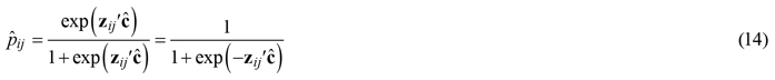
In the ingrowth model, it is assumed that the number of ingrowth trees is distributed according to zero-inflated negative binomial distribution. Negative binomial distribution gave better results than Poisson distribution because the counts had a larger variance than implied by Poisson distribution. The zero-inflated negative binomial distribution is a discrete distribution having density function f

where k is the number of counts, g is the negative binomial density function, p is the probability of extra zeros, µ is the mean of distribution g and α is the dispersion parameter so that the variance of g is μ + αμ2. The extra-zero probability p is needed if there are more zeros in the data than implied by the distribution g. It cannot be determined for an individual zero whether it an extra-zero or an “ordinary” zero. The probability that a zero is an extra zero is ![]() When α = 0, the distribution is the Poisson distribution, which has the variance µ. Often the dispersion parameter is defined as
When α = 0, the distribution is the Poisson distribution, which has the variance µ. Often the dispersion parameter is defined as ![]() We prefer α as it increases when dispersion increases.
We prefer α as it increases when dispersion increases.
The density function of the negative binomial distribution is:

The mean and variance of f are (Zuur et al. 2012):
![]()
![]()
Note that the mean does not depend on α. The variance can be derived using the formula ![]() now the conditioning variable is the random indicator variable telling whether the observation is an extra zero.
now the conditioning variable is the random indicator variable telling whether the observation is an extra zero.
For the ingrowth of period j in stand i, µ is related to a linear predictor via log-link:
![]()
where xij is the vector of independent variables, a is a fixed parameter vector and ![]() is a random effect. According to (5), µij is a lognormally distributed random variable. However, in Eqs. 3 and 4, µ needs to be interpreted as the conditional mean given the random effect. The model for counts that are not extra zeros is called the count model. The first variable in xij is 1, i.e., a1 is the intercept. Also, such models will be considered where the random effect is missing. Such models proved to be more useful.
is a random effect. According to (5), µij is a lognormally distributed random variable. However, in Eqs. 3 and 4, µ needs to be interpreted as the conditional mean given the random effect. The model for counts that are not extra zeros is called the count model. The first variable in xij is 1, i.e., a1 is the intercept. Also, such models will be considered where the random effect is missing. Such models proved to be more useful.
Eq. 5 means that
![]()
When using Eq. 6 to predict a typical count, the random effect bi is taken to be zero, and the predictor of y is
![]()
The same predictor is also used in the fixed-effects model where the random effect b is missing. The expected value of yij is another possible predictor. Recall that for a lognormally distributed variable ![]() where μ' and σ are the mean and standard deviation of log(X), respectively. Thus
where μ' and σ are the mean and standard deviation of log(X), respectively. Thus ![]() and
and ![]() As µ is a lognormally distributed variable, we get an unbiased predictor for yij using its expected value:
As µ is a lognormally distributed variable, we get an unbiased predictor for yij using its expected value:
![]()
The variance of yij is obtained using again the formula ![]() where
where
![]()
is obtained from Eq. 4, and
![]()
is obtained from Eq. 3. ![]() is used to compute Pearson residuals.
is used to compute Pearson residuals.
Two predictor variables are of special interest: the time interval over which the ingrowth trees are appearing and the plot size. In the literature, these variables are called exposure variables (Baetschmann and Winkelmann 2012; Mehtätalo and Lappi 2020). A natural assumption is that the expected number of ingrowth counts is proportional to both exposure time and the plot size. We assume that the expected number of counts is always proportional to the plot size in a given stand. Concerning the exposure time, the proportionality assumption is more questionable. The proportionality assumption was studied by merging consecutive observations in the same plot.
The assumption that the expected counts are proportional to both exposure time and plot size can be made using the exposure time Tij, and the plot size Aij as offset variables, i.e., we can estimate the model
![]()
Note that Eq. 11 can be used also in prediction for other exposure times and plot sizes. In the merged data set with two exposure times, we add log(Tij) among the predictor variables and thus we estimated model
![]()
using only log(A) as the offset. Note that according to Eq. 12, μ is proportional to Tγ. The estimate of γ is compared to one.
The probability that yij is an extra zero is modeled via logit-link:

Again, it is assumed that the first variable in zij is 1, i.e., c1 is the intercept. It is assumed that the model for extra zeros does not depend on the exposure time or plot size. This assumption guarantees that the expected number of counts is proportional to the exposure time and plot size, if they are proportional in the count model.
After estimating the parameter vector c of model (13), we can predict the extra-zero probability pij using the logistic function, i.e.
Thereafter, the expected number of ingrowth trees yij is estimated using (7) or (8), and the variance is estimated using (4) or (9) + (10). Using these estimates we computed Pearson residuals defined as the difference between observed count and predicted count divided by the standard deviation.
We are interested in ingrowth in the connection of continuous cover forestry where sufficient gradual regeneration is necessary for the sustainability of the method. However, an excessive number of ingrowth trees is not a benefit as only a limited number of new trees have sufficient growing space and can be grown to merchantable tree sizes. Thus, we analyze also the right-censored ingrowth variable y(K) = min(y,K). K was taken as 5 (500 trees per hectare in five years).
For the ingrowth of period j in plot i, let us denote the probability that yij = k by fijk. For the fixed effects model, fijk can be computed using (1). When there is a random plot effect in the model, the probabilities fijk can be computed as follows:

where h is the normal density with mean 0and variance σ2. We did the integration by simulating 10 000 observations from the normal distribution (R function “integrate” could be also used). When the above equations are applied using the estimated parameters, the equalities are only approximate, e.g., Eq. 8 is only approximately unbiased.
The probability that yij(K) = K is denoted by fij(K) and computed as ![]() The goodness-of-fit of the estimated marginal distribution is described with the statistic
The goodness-of-fit of the estimated marginal distribution is described with the statistic

where Ok is the number of observations having yij = k, O(K) is the number of observations having yij ≥ K, Ek is the expected number of observations having yij = k, i.e. ![]() and E(K) is the expected number of observations having yij ≥ K, i.e.
and E(K) is the expected number of observations having yij ≥ K, i.e. ![]() where ni is the number of measurements for plot i. We note further that
where ni is the number of measurements for plot i. We note further that


The Pearson residuals of yij(K) were computed using Eqs. 17–19.
Models without random effects were estimated using the zeroinfl function in R package pscl (Jackman 2017). Models with random effects were estimated using the glmmTMB function in R package glmmTMB (Brooks et al. 2017). In these packages the dispersion parameter is θ = 1/α.
As potential predictor variables, we used species group-specific variables or variables computed using all trees. We used the basal area, logarithm of basal area augmented by a small constant (0.01) and square root of basal area. In addition, site type dummies and temperature sum were used as potential predictors. Some nonsignificant predictors were kept in the models if they make the models more logical. Models with these predictors can be compared with the models of Pukkala et al. (2013). Also, basal-area-weighted mean diameter and its square, the standard deviation of the diameter distribution and the skewness of the diameter distribution would be significant predictors, but models with them would be more problematic in practical predictions and could not be compared with the earlier models.
4 Results
We developed the count models both without (Tables 1–3) and with (Tables 5–7) random plot effects. The right-censoring limit K was given value 5 when analyzing 5 years’ growth periods, corresponding to 500 trees per hectare in 5 years. Table 4 presents prediction statistics when fixed-effects models are used. Table 8 presents the statistics for the mixed-effects models.
| Table 1. The fixed-effects ingrowth model for Scots pine estimated with the zeroinfl function in R package pscl. The function estimates the dispersion parameter in form log(1/α). G is the stand basal area, VT and CT are the indicator variables for sub-xeric and xeric or poorer forest types. Log(T) and log(A) are used as offsets, where A = 100 m2 is the area of plot and T = 5 yrs is the length of the growth period. | |||
| Predictor | Estimate | Std. Error | Pr(>|z|) |
| Count model (negative binomial with log link) | |||
| log(T) | 1 | ||
| log(A) | 1 | ||
| Intercept | –6.82 | 0.41 | <2e–16 |
| Gpine | –0.131 | 0.112 | 0.023 |
| 0.783 | 0.308 | 0.011 | |
| VT | 0.633 | 0.250 | 0.011 |
| CT | 1.64 | 0.34 | 1.2e–06 |
| ln(1/α) | –1.16 | 0.209 | |
| Zero-inflation model coefficients (binomial with logit link) | |||
| Intercept | –13.6 | 3.5 | 0.0001 |
| ln(Gpine + 0.01) | –0.307 | 0.083 | 0.00021 |
| √G | 6.1 | 1.5 | 5.9E–05 |
| G | –0.58 | 0.16 | 0.0003 |
| VT | –1.21 | 0.36 | 0.00075 |
| α = 3.19; Log-likelihood –905.2 on 11 degrees of freedom. | |||
| Table 2. The fixed-effects ingrowth model for Norway spruce. OMT is an indicator variable for herb-rich or better site. TS is the temperature sum. The other symbols are as in Table 1. | |||
| Predictor | Estimate | Std. Error | Pr(>|z|) |
| Count model (negative binomial with log link) | |||
| log(T) | 1 | ||
| log(A) | 1 | ||
| Intercept | –6.61 | 0.54 | <2e–16 |
| log(Gspruce + 0.01) | 0.148 | 0.029 | 2.9e–07 |
| max(Gspruce – 13.0) | –0.0207 | 0.0109 | 0.056 |
| TS | 0.00126 | 0.00048 | 0.0082 |
| log(1/α) | –0.83 | 0.11 | |
| Zero-inflation model coefficients (binomial with logit link) | |||
| Intercept | –1.75 | 0.46 | 8.6e–05 |
| log(Gspruce + 0.01) | –0.359 | 0.073 | 9.0e–07 |
| OMT | 1.12 | 0.43 | 0.0085 |
| CT | 1.10 | 0.48 | 0.021 |
| α = 2.28; Log-likelihood –22987 on 9 degrees of freedom. | |||
| Table 3. The fixed-effects ingrowth model for birch (combined ingrowth of silver and downy birch). The symbols are as in Table 1. | |||
| Predictor | Estimate | Std. Error | Pr(>|z|) |
| Count model (negative binomial with log link) | |||
| log(T) | 1 | ||
| log(A) | 1 | ||
| Intercept | –3.15 | 0.18 | <2e–16 |
| Gpine | 0.0923 | 0.0090 | <2e–16 |
| Gbirch | –0.109 | 0.045 | 0.016 |
| √Gbirch | 0.349 | 0.150 | 0.020 |
| G | –0.113 | 0.0091 | <2e–16 |
| VT | –0.50 | 0.16 | 0.0016 |
| CT | –0.87 | 0.29 | 0.0032 |
| log(1/α) | –1.013 | 0.092 | |
| Zero-inflation model (binomial with logit link) | |||
| Intercept | –6.40 | 1.57 | 0.000044 |
| log(Gbirch + 0.01) | –0.565 | 0.17 | 0.00078 |
| G | 0.142 | 0.033 | 0.000014 |
| VT | 0.822 | 0.51 | 0.11 |
| CT | 2.41 | 0.75 | 0.0014 |
| α = 2.57; Log-likelihood –2700 on 13 degrees of freedom. | |||
In the dataset where observations within the same plot were merged, we estimated models where log(T) was used either as a predictor or as an offset. The likelihood ratio test indicated that the coefficient of log(T) did not differ from one neither in models with random effects nor in models without random effects. Therefore, we do not present any further results for the merged data set.
According to Table 4, the models fitted without random effects had very small biases (–0.0016 for pine, 0.010 for spruce and 0.12 for birch). However, the coefficients of determination were rather modest: 0.086 for pine, 0.052 for spruce and 0.154 for birch. The distributions of the residuals were very skew: the proportions of positive residuals were 0.11, 0.27 and 0.25 for pine, spruce and birch, respectively. The means of Pearson residuals were close to zero and the standard deviations were close to one. The overdispersion parameter α was large for all species (between 2.28 and 3.19) indicating large overdistribution. The right-censored variable yij(K) was predicted without bias. The coefficient of determination was 0.17 for pine, 0.11 for spruce and 0.18 for birch. The prediction variance was well estimated using Eq. 19 as can be seen from the fact that the Pearson residuals had standard deviations close to one.
| Table 4. Statistics for the fixed-effects ingrowth models. Row “P(Residual > 0)” gives the proportion of positive residuals. | ||||
| Variable | Minimum | Maximum | Mean | sd |
| Scots pine | ||||
| Ingrowth | 0 | 68 | 0.90 | 4.07 |
| Censored ingrowth | 0 | 5 | 0.457 | 1.26 |
| Probability of extra zeroes (p) | 0.0009 | 0.97 | 0.68 | 0.28 |
| Prediction | 0.018 | 8.10 | 0.890 | 1.38 |
| Residual | –8.10 | 64.34 | –0.0016 | 3.89 |
| P(Residual > 0) | 0.11 | |||
| Pearson residual | –0.55 | 28.79 | –0.0020 | 1.13 |
| Censored prediction | 0.017 | 2.39 | 0.47 | 0.52 |
| Censored residual | –2.37 | 4.90 | –0.001 | 1.15 |
| Censored Pearson residual | –1.05 | 9.91 | –0.007 | 0.93 |
| Norway spruce | ||||
| Ingrowth | 0 | 47 | 2.61 | 5.3 |
| Censored ingrowth | 0 | 5 | 1.47 | 1.95 |
| Probability of extra zeroes (p) | 0.04 | 0.74 | 0.22 | 0.20 |
| Prediction | 0.27 | 5.0 | 2.60 | 1.29 |
| Residual | –4.84 | 43.6 | 0.010 | 5.16 |
| P(Residual > 0) | 0.27 | |||
| Pearson residual | –0.61 | 12.97 | 0.0010 | 1.08 |
| Censored prediction | 0.24 | 2.27 | 1.49 | 0.59 |
| Censored residual | –2.25 | 4.71 | –0.022 | 1.84 |
| Censored Pearson residual | –1.04 | 4.97 | –0.014 | 0.98 |
| Birch (silver birch and downy birch) | ||||
| Ingrowth | 0 | 120 | 5.45 | 12.8 |
| Censored ingrowth | 0 | 5 | 1.77 | 2.14 |
| Probability of extra zeroes (p) | 0.0015 | 0.940 | 0.17 | 0.21 |
| Prediction | 0.035 | 23.4 | 5.33 | 4.29 |
| Residual | –19.4 | 102.7 | 0.12 | 11.7 |
| P(Residual > 0) | 0.25 | |||
| Pearson residual | –0.60 | 11.4 | –0.0023 | 1.02 |
| Censored prediction | 0.035 | 3.31 | 1.75 | 0.80 |
| Censored residual | –3.19 | 4.48 | 0.023 | 1.95 |
| Censored Pearson residual | –1.47 | 6.03 | 0.0098 | 1.00 |
The probability that yij is an extra zero was negatively correlated with the expected value of yij given that it is not an extra zero. The correlation between the linear predictor (5) (where bi was taken to be zero) of the count model and the linear predictor of the zero-inflation model was –0.68, –0.82 and –0.29 for pine, spruce and birch, respectively. The average probability of extra zeros was 0.68, 0.22 and 0.21, for pine, spruce and birch, respectively. The average expected counts were 0.90 (pine), 2.60 (spruce) and 5.33 (birch), thus also showing the negative association between the number of extra zeros and the expected number of ingrowth trees.
The model for pine predicts that pine ingrowth is the most abundant with stand basal area of 5–7 m2 ha–1 (Fig. 1). Ingrowth is the most plentiful on xeric sites. Admixtures of spruce and birch decrease the ingrowth of pine. In the model for spruce, the temperature sum has a strong effect on the prediction, ingrowth decreasing toward northern latitudes where the temperature sum is lower. The model predicts that maximum ingrowth is obtained for stand basal area 13 m2 ha–1. The decrease of ingrowth for high basal areas is implied by the predictor max(Gspruce–13.0), which is kept in the model even if its p-value is slightly greater than 0.05 to obtain a more logical model. The amount of ingrowth does not depend on the presence of other tree species in the stand. Birch ingrowth decreases with increasing stand balsa area and towards lower fertility classes. The presence of pine increases birch ingrowth.
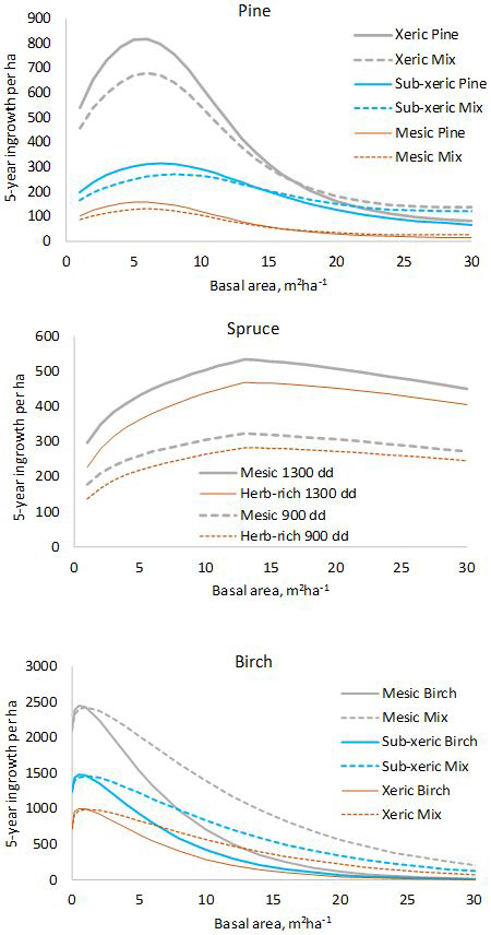
Fig. 1. Five-year predictions calculated with the fixed-effects model shown in Tables 1–3. log(10000) and log(5) were used as offsets to obtain per-hectare values for five years. In the diagram for pine, “Mix” refers to a stand where 50% of the basal area is pine and 50% is other species. In the diagram for birch, “Mix” is a stand where 50% of the basal area is birch and 50% is pine.
We then estimated models having random plot effects in the count models (Tables 5–7). When there were random effects in the count model, the best zero-inflation model contained fewer significant predictors (pine only intercept) and the average extra-zero probabilities were smaller. Without random effects, the average extra-zero probabilities were 0.68 (pine), 0.22 (spruce) and 0.21 (birch) while in the models with random effects the average probabilities were 0.0045 (pine), 0.042 (spruce) and 0.055 (birch) (Table 8). With random effects, the dispersion parameter α was smaller. For the spruce, the dispersion parameter was so small that the estimated model is practically equivalent to a zero-inflated Poisson model. The random effects describe overdistribution, which otherwise is described with large α.
| Table 5. The mixed-effects ingrowth model for Scots pine. VT is the sub-xeric type, and CT is the xeric type. | |||
| Predictor | Estimate | Std. Error | Pr(>|z|) |
| Conditional model | |||
| log(T) | 1 | ||
| log(A) | 1 | ||
| Intercept | –6.47 | 0.56 | <2e–16 |
| ln(Gpine + 0.01) | 0.323 | 0.074 | 1.4E–05 |
| √G | –1.04 | 0.13 | 6.4E–15 |
| VT | 0.73 | 0.23 | 0.0018 |
| CT | 1.23 | 0.37 | 0.00082 |
| Zero-inflation model | |||
| Intercept | –5.40 | 0.88 | 8.6e–10 |
| α = 0.135; σ = 3.06; Log-likelihood = –820.6 on 7 Df. | |||
| Table 6. The mixed-effects ingrowth model for Norway spruce. TS is the temperature sum and CT is the xeric type. | |||
| Predictor | Estimate | Std. Error | Pr(>|z|) |
| Count model | |||
| log(T) | 1 | ||
| log(A) | 1 | ||
| Intercept | –7.58 | 0.69 | <2e–16 |
| ln(Gspruce + 0.01) | 0.287 | 0.032 | <2e–16 |
| max(Gspruce – 13.0) | –0.0532 | 0.0126 | 2.4e–05 |
| LS | 0.000716 | 0.00060 | 0.235 |
| Zero-inflation model | |||
| Intercept | –3.74 | 0.27 | <2e–16 |
| ln(Gspruce + 0.01) | –0.32 | 0.12 | 0.0096 |
| CT | 1.31 | 1.02 | 0.20 |
| α = 0.0071; σ = 1.79; Log-likelihood = –2156.2. | |||
| Table 7. The mixed-effects ingrowth model for birch. | |||
| Predictor | Estimate | Std. Error | Pr(>|z|) |
| Conditional model | |||
| log(T) | 1 | ||
| log(A) | 1 | ||
| Intercept | –4.27 | 0.20 | <2e–16 |
| G | –0.127 | 0.010 | <2e–16 |
| log(Gbirch + 0.01) | 0.221 | 0.030 | 1.6e–13 |
| Gpine | 0.0815 | 0.0107 | 2.7e–14 |
| CT | –0.21 | 0.19 | 0.26 |
| Zero-inflation model | |||
| Intercept | –5.03 | 0.86 | 4.2e–09 |
| G | 0.0929 | 0.033 | 0.004 |
| α = 0.101; σ = 2.056; Log-likelihood = –2615.2. | |||
| Table 8. Statistics for the mixed-effects ingrowth models. Notations (11) and (12) refer to Eqs. 11 and 12, respectively. | ||||
| Variable | min | max | mean | sd |
| Scots pine | ||||
| Probability of extra zeroes (p) | 0.0045 | 0.0045 | 0.0045 | 0 |
| Prediction | 0.0001 | 0.767 | 0.039 | 0.072 |
| Prediction | 0.010 | 82.91 | 4.21 | 7.84 |
| Residual (11) | –0.6668 | 67.87 | 0.8567 | 4.05 |
| P(Residual (11) > 0) | 0.16 | |||
| Residual (12) | –72.12 | 54.48 | –3.318 | 7.60 |
| P(Residual(12) > 0) | 0.055 | |||
| Pearson residual (11) | –8.01E–05 | 0.260 | 0.002 | 0.012 |
| Pearson residual (12) | –0.0087 | 0.252 | –0.007 | 0.012 |
| Censored prediction | 0.0075 | 1.86 | 0.390 | 0.335 |
| Censored residual | –1.80 | 4.83 | 0.068 | 1.17 |
| Censored Pearson residual | –0.84 | 6.80 | 0.019 | 0.94 |
| Norway spruce | ||||
| Probability of extra zeroes (p) | 0.0068 | 0.277 | 0.042 | 0.060 |
| Prediction | 0.090 | 1.37 | 0.695 | 0.382 |
| Prediction | 0.45 | 6.83 | 3.47 | 1.90 |
| Residual (11) | –1.30 | 46.27 | 1.91 | 5.25 |
| P(Residual(11) > 0) | 0.43 | |||
| Residual (12) | –6.47 | 43.37 | –0.86 | 5.20 |
| P(Residual(12) > 0) | 0.24 | |||
| Pearson residual (11) | –0.040 | 6.560 | 0.12 | 0.39 |
| Pearson residual (12) | –0.20 | 6.41 | –0.038 | 0.39 |
| Censored prediction | 0.33 | 2.07 | 1.34 | 0.54 |
| Censored residual | –2.02 | 4.64 | 0.13 | 1.85 |
| Censored Pearson residual | –0.99 | 4.81 | 0.070 | 1.07 |
| Birch (silver birch and downy birch) | ||||
| Probability of extra zeroes (p) | 0.0074 | 0.45 | 0.055 | 0.050 |
| Prediction (11) | 0.0070 | 5.50 | 1.18 | 1.09 |
| Prediction (12) | 0.058 | 45.5 | 9.79 | 9.00 |
| Residual (11) | –5.23 | 117.2 | 4.27 | 12.4 |
| P(Residual(11) > 0) | 0.43 | |||
| Residual (12) | –43.3 | 96.7 | –4.35 | 12.9 |
| P(Residual(12) > 0) | 0.18 | |||
| Pearson residual (11) | –0.014 | 2.30 | 0.057 | 0.17 |
| Pearson residual (12) | –0.12 | 2.20 | –0.041 | 0.17 |
| Censored prediction | 0.052 | 3.27 | 1.63 | 0.75 |
| Censored residual | –3.22 | 4.57 | 0.142 | 1.98 |
| Censored Pearson residual | –1.55 | 4.81 | 0.080 | 1.07 |
We also estimated such models where the random effects varied from measurement to measurement. Note that models with observation level random effects can be estimated using generalized linear mixed models contrary to ordinary linear mixed-effects models (p. 279 in Mehtätalo and Lappi 2020). These models were clearly worse than the models where the same random effect applies to all remeasurements of the same plot.
The log-likelihoods indicated that the models with random effects would be always better. However, the models with random effects are problematic in the prediction. The predictor of the typical value produces underestimates of yij, as it should do, but predictor (8), which should provide approximately unbiased predictions, is producing clearly too large predictions. The proportions of the positive residuals are closer to 0.5 using predictor (7) than using the same predictor in fixed-effects models. Using predictor (8) the proportions of positive residuals are smaller than in the fixed-effects models. The variances obtained from Eqs. 9 and 10 are clearly too large so that the standard deviations of the Pearson residuals are small. However, the censored predictions are not so biased, and the standard deviations of the Pearson residuals are close to 1.
The empirical and theoretical distributions (Fig. 2) were compared with χ2 statistic (Eq. 16). For the fixed-effects model of pine, χ2 was 2.99 (df = 6, p = 0.81). For the mixed-effects model, the value was χ2 = 15.80 (p = 0.015). In the model for spruce, χ2 was 4.02 (p = 0.67) for the fixed-effects model, and for the mixed effect model χ2 was 21.7 (p = 0.0014). For birch, the values were; χ2 = 3.71 (p = 0.71) for fixed-effects model and χ2 = 39.3 (p < 0.0001) for mixed-effects model. Thus the observed marginal distributions agree perfectly with the predicted distributions for fixed-effects models, but the agreement is poor for the mixed-effects models.
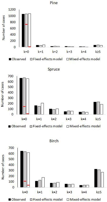
Fig. 2. Number of plots with 0, 1, 2, 3, 4 or ≥5 ingrowth trees based on observed and predictedingrowth. The marginal distribution of the predicted ingrowth is computed using Eq. 1. The frequency of extra zeros is shown with the red horizontal line.
5 Discussion
The zero-inflated negative binomial (ZINB) distribution is commonly used to model count data, which is overdispersed compared to the Poisson model and which has more zeros than implied by the negative binomial model. There is software available for fitting ZINB models in the framework of generalized linear (mixed) models. We used ZINB models to describe ingrowth in the permanent sample plots of the Finnish national forest inventory. Ingrowth models are important in most silvicultural systems but especially when analyzing the possibilities of continuous cover forestry.
The predictions of the fixed-effects models of this study are unbiased while predictions of models developed with a different method (Pukkala et al. 2013) are clearly biased. The average ingrowth in the data was 90, 261 and 545 trees/ha in 5 years for pine, spruce and birch, respectively. The average predictions of our models were 90, 260 and 533 trees/ha in 5 years for the fixed-effects model. The average predictions using the models of Pukkala et al. (2013) were 12, 62 and 276 trees/ha in 5 years. When considering the prediction of ingrowth using the models of this study in practice, it may be reasonable to use the estimator of ![]() instead of estimator of
instead of estimator of ![]() Using the fixed-effects estimator of
Using the fixed-effects estimator of ![]() the unbiased average predictions were 47, 149 and 175 trees/ha in 5 years.
the unbiased average predictions were 47, 149 and 175 trees/ha in 5 years.
Pukkala et al. (2013) estimated their models using data that contained two additional data sets that were not used in this study. The additional data sets had plot areas 300 m2 and 1600 m2. When they estimated the models for the probability of ingrowth, they ignored the differences in plot areas. When they estimated the amount of ingrowth in plots having ingrowth, they converted the ingrowth numbers to per hectare values. They used logarithmic regression for the amount of ingrowth in the plots having ingrowth. When transforming logarithmic predictions back to the arithmetic scale they corrected the back-transformation bias by adding half of the logarithmic residual variance to the logarithmic prediction before applying the exp-function. However, the residual variance is dependent both on the plot area and on the expected stand density. Because the exponential function is convex, the use of the average residual variance leads on average to too small predictions.
In addition, the ingrowth was lower in the two additional datasets used in Pukkala et al. (2013) than in the NFI data set used in this study. The influence of the additional data sets was increased by the fact that they used weighted regression in the ingrowth model, the weight being proportional to the plot area. Using their models, the proportions of the positive residuals were 0.23, 0.46 and 0.35 for pine, spruce and birch, respectively. These figures are closer to 0.5 than using the models of this study in all cases except when predictor (7) is used in the mixed model for birch. Thus, their models can be justified from the viewpoint of predicting median ingrowth instead of the mean. The shapes of the prediction functions can be compared between these two studies. Compared to the earlier model, the predictions of our new fixed-effects model for pine resemble those of the earlier model and the number of ingrowth trees on the major growing site of pine (sub-xeric) is similar with both models when the stand basal area is 5–15 m2 ha–1. The earlier model predicts maximum ingrowth for stand basal area of about 3 m2 ha–1 whereas our new model gives the highest predictions for 5–7 m2 ha–1. Both models predict clearly lower ingrowth for mesic (MT) or herb-rich (OMT), compared to sub-xeric site (VT), which have smaller ingrowth than xeric sites (CT).
The fixed-effects model for spruce predicts maximal ingrowth when the basal area of spruce is 13 m2 ha–1 whereas the earlier model predicts maximal ingrowths at 5 m2 ha–1, after which ingrowth decreases slowly with increasing stand basal area. Plotting the ingrowth and basal area of spruce shows much irregularity in the middle range of the basal area. Furthermore, there are two observations with large basal area and large ingrowth. Opposite to the previous model, our model does not predict increasing spruce ingrowth with increasing admixture of pine. Increasing temperature sum increase ingrowth prediction, which is logical since the interval between prolific seed years increases towards the north, and the growth rate of seedlings is slower in the north.
The difference between the predictions of the old model and our new fixed-effects model was the smallest for birch ingrowth. The average predicted ingrowth was still almost twice as large as in the old model. The overall effect of the basal area is the same in both models, and the presence of pine increases ingrowth in both models.
The expected number of ingrowth trees in a plot during a specific period is evidently dependent on the plot area and the length of the period. A natural assumption is that the expected number of ingrowth trees is proportional to the plot area. This assumption can be described in a ZINB model by using the logarithm of the plot area as an offset in the logarithmic model as expressed in Eqs. 11 and 12. Concerning the exposure time, the proportionality assumption is more questionable. We tested this assumption in the dataset where two consecutive 5 years’ growth periods were merged whenever possible. It was found that the coefficient of log(T) did not deviate significantly from one in Eq. 12. However, it is not logical to assume that the same model having log(T) as an offset would be valid for much longer periods than 10 years because there are dynamic predictors in Eq. 11 which change over time.
When the species-specific basal-area-weighted mean diameter and its square were added as predictors to the count models, they were statistically significant. The models indicated large ingrowth for small mean diameters, especially for spruce and birch. These models are not presented, because they are problematic in predictions: they imply that ingrowth is large if the ingrowth is large. Also, the standard deviation and skewness of the diameter distribution of all trees would be statistically significant predictors especially in interaction with mean diameter.
The expected number of ingrowth trees is not the only, and perhaps not the most important, variable of interest concerning regeneration in continuous cover forestry. Also, the spatial pattern of ingrowth trees affects the regeneration result. If there are locally more trees than needed for sufficient regeneration, the extra trees cannot completely compensate for the gaps. Thus we also analyzed how the models predicted a right-censored variable min(y,5). The analysis of the right-censored variable cannot be directly generalized for other plot sizes. For instance, the expected value of min(y,5) is not proportional to the plot area. The prediction of min(y,5) was based on the assumption that 500 ingrowth trees/ha is sufficient regeneration for a plot size of 100 m2. Of course, having 500 ingrowth trees/ha in 5 years overall in the forest is more than sufficient, but extra trees in a 100 m2 plot may be needed to compensate for neighboring gaps. Having two ingrowth trees in a plot of 40 m2 implies also 500 trees/ha, but min(y,2) in a 40 m2 plot has a smaller expected value computed per ha than min(y,5) in a 100 m2 plot. The density 500 trees/ha is obtained in a plot with A m2, if there are ![]() trees in the plot. The dependency of the expected value of
trees in the plot. The dependency of the expected value of ![]() on A is shown in Fig. 3 when using models without random effects (Tables 1–3). When the plot area increases, the number of accepted trees per ha increases, but only very slightly. The slight increase is related to the fact that when the plot area increases, the variance increases even more (see Eq. 4). The average probability of censoring also increases with increasing plot area when the acceptable limit for ingrowth is 500 trees/ha in 5 years (Fig. 3 right). This surprising result is related to the implied spatial distribution. If the distribution of the number of ingrowth trees would have the same mean function and the same probability of extra zeros but α would be zero, i.e. the distribution would be Poisson, then the probability of censoring would still increase for birch, but for spruce, the probability would decrease after a short increase. For pine, the probability would be practically constant.
on A is shown in Fig. 3 when using models without random effects (Tables 1–3). When the plot area increases, the number of accepted trees per ha increases, but only very slightly. The slight increase is related to the fact that when the plot area increases, the variance increases even more (see Eq. 4). The average probability of censoring also increases with increasing plot area when the acceptable limit for ingrowth is 500 trees/ha in 5 years (Fig. 3 right). This surprising result is related to the implied spatial distribution. If the distribution of the number of ingrowth trees would have the same mean function and the same probability of extra zeros but α would be zero, i.e. the distribution would be Poisson, then the probability of censoring would still increase for birch, but for spruce, the probability would decrease after a short increase. For pine, the probability would be practically constant.
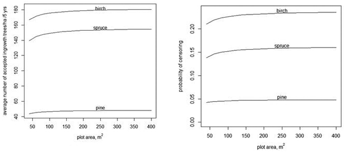
Fig. 3. The average number of accepted ingrowth trees per ha when the censoring limit is 500 trees per ha, i.e., the censored variable is min(y,![]() ) (left) and the average probablity that some ingrowth trees within a plot are censored when 500 trees/ha are accepted (right).
) (left) and the average probablity that some ingrowth trees within a plot are censored when 500 trees/ha are accepted (right).
When the number of acceptable trees increases in a 100 m2 plot, the average number of acceptable trees per hectare also increases (Fig. 4, left) and the probability of censoring decreases (Fig. 4, right).
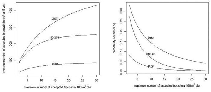
Fig. 4. Average number of acceptable ingrowth trees/ha in 5 years (left) and the probability that some trees are censored in a 100 m2 plot (right) as a function of the maximum number of acceptable trees in a 100 m2 plot. As a reference, note that without censoring there are 90, 259 and 524 trees/ha for pine, spruce and birch, respectively (see the "Prediction" rows of Table 4).
We used logit-link in the zero-inflation part of the model, i.e., in Eq. 13 , as is usually done. However, Baetschmann and Winkelmann (2012) give theoretical reasons for using a complementary log-log link. In this study logit link gave slightly better results.
The results of this study indicated that the models estimated without random plot effects were quite unbiased for the prediction of the ingrowth. The predictions had very small biases in terms of ordinary and Pearson residuals, and the standard deviations of Pearson residuals were close to one. The marginal distribution of counts agreed very well with the theoretical distributions.
The most problematic feature of the current analysis is that models with random plot effects seemed to fit the data better, in terms of the likelihood, than the models without random effects. However, the implied theoretically unbiased predictions were clearly biased. Also, the implied marginal distribution of the predicted counts did not fit the data. Without the random effects, the theoretical and empirical marginal distributions agreed almost perfectly (Fig. 2). There are two possible reasons for the problems with the mixed-effects models. First, the distribution of the random effect in the linear predictor (11) may be far from the normal distribution. Second, the assumed negative binomial distribution may not be valid. Recall that the censored predictions were quite unbiased and their estimated variances produced Pearson residuals having standard deviations close to one. Thus the problems are related to the large values of random effects. It may be that modeling without random effects is more robust concerning model misspecification. Note that both models, with and without random effects, implied very large overdispersion compared to the fixed-effect Poisson model. It should also be kept in mind that ingrowth values in the data were not exact measurements but were obtained using initial counts and final counts and the mortality models.
The large variability of ingrowth is both a theoretical and practical problem in continuous cover forestry. In practice, the managers should be able to react properly, when the ingrowth is not sufficient. In theoretical calculations providing management rules and comparisons with even-aged forestry, deterministic simulations using expected values of ingrowth are highly misleading. The expected values of censored ingrowth, provided by the models of this study, provide a better, but not yet sufficiently good basis. Stochastic simulations using the distributions obtained from the estimated models are, however much more demanding than deterministic simulations. One problem in stochastic simulations is for what plot size the simulations should be done, or should a stand be constructed from several plots. When generalizing our models to other plot sizes, it sounds reasonable to assume that the expected number of counts is proportional to the plot area. However, it is possible that different overdispersion parameters α give optimal description for the ingrowth, in terms of the negative binomial distribution, for different plot sizes. If mixed-effect models are used, it is not clear whether random plot effects can be interpreted as random stand effects.
The probability of extra zero is according to our model the proportion of stands having zero ingrowth whatever is the plot size and exposure time. As it is estimated from 100 m2 plots and 5 years exposure times, it should not be interpreted too literally but anyhow it describes the proportion of stands with very small ingrowth. In mixed models, the extra zero probabilities are very small, and stands with very small ingrowth are obtained having small random effects in the count model, if random effects are interpreted as stand effects.
Planning of continuous cover forestry methods cannot be based directly on the ingrowth models of this study. For instance, seed production, which is a prerequisite of ingrowth, requires the presence of rather large trees in the stand or its surroundings (Nygren et al 2017). The size distribution of trees was not taken into account in our modeling. An admixture of pine and birch in a spruce stand often enhances the regeneration and ingrowth of spruce (Pukkala et al. 2013), but this effect was not included in our models. Soil type may also have a strong influence on regeneration and ingrowth.
Acknowledgements
Lauri Mehtätalo and two anonymous referees made useful comments.
References
Baetschmann G., Winkelmann R. (2012). Modelling zero-inflated count data when exposure varies: with an application to sick leave. University of Zurich Department of Economics Working Paper 61. 16 p. https://doi.org/10.2139/ssrn.2005793.
Brooks M.E., Kristensen K., van Benthem K.J., Magnusson A., Berg C.W., Nielsen A., Skaug H.J., Maechler M., Bolker B.M. (2017). glmmTMB balances speed and flexibility among packages for zero-inflated generalized linear mixed modeling. The R Journal 9(2): 378–400. https://doi.org/10.32614/RJ-2017-066.
Hynynen J., Ojansuu R., Hökkä H., Siipilehto J., Salminen H., Haapala P. (2002). Models for predicting stand development in MELA system. The Finnish Forest Research Institute Research Papers 835. 116 p. http://urn.fi/URN:ISBN:951-40-1815-X.
Jackman S. (2017). Package “pscl”. http://github.com/atahk/pscl.
Mehtätalo L., Lappi J. (2020). Biometry for forestry and environmental data with examples in R. CRC Press Taylor and Francis group. 411 p. https://doi.org/10.1201/9780429173462.
Miina J., Pukkala T. (2000). Using numerical optimization for specifying individual-tree competition models. Forest Science 46(2): 277–283.
Nikula A., Nivala V., Matala J., Heliövaara K. (2019). Modelling the effect of habitat composition and roads on the occurrence and number of moose damage at multiple scales. Silva Fennica 53(1) article 9918. https://doi.org/10.14214/sf.9918.
Nygren M., Rissanen K., Eerikäinen K., Saksa T., Valkonen S. (2017). Norway spruce cone crops in uneven-aged stands in southern Finland: a case study. Forest Ecology and Management 390: 68–72. https://doi.org/10.1016/j.foreco.2017.01.016.
Pukkala T., Lähde E., Laiho O. (2009). Growth and yield models for uneven-sized forest stands in Finland. Forest Ecology and Management 258(3): 207–216. https://doi.org/10.1016/j.foreco.2009.03.052.
Pukkala T., Lähde E., Laiho O. (2013). Species interactions in the dynamics of even- and uneven-aged boreal forests, Journal of Sustainable Forestry 32(4): 371–403. https://doi.org/10.1080/10549811.2013.770766.
Pukkala T., Lähde E., Laiho O. (2014). Stand management optimization – the role of simplifications. Forest Ecosystems 1 article 3. 11 p. https://doi.org/10.1186/2197-5620-1-3.
Stroup W.W. (2013). Generalized linear mixed models. Modern concepts, methods and applications. 1st edition. CRC Press Taylor and Francis group, Boca Raton. 529 p.
Vanclay J. (1994). Modelling forest growth and yield: applications to mixed tropical forests. CAB International, Wallingford, UK. 312 p. ISBN 0-85198-913-6.
Zuur A.F., Saveliev A.A, Ieno E.N. (2012). Zero inflated models and generalized linear mixed models with R. Highland Statistics Ltd. 323 p.
Total of 14 references.
