Kenneth Olofsson  ,
Johan Holmgren
,
Johan Holmgren
Co-registration of single tree maps and data captured by a moving sensor using stem diameter weighted linking
Olofsson K., Holmgren J. (2022). Co-registration of single tree maps and data captured by a moving sensor using stem diameter weighted linking. Silva Fennica vol. 56 no. 3 article id 10712. https://doi.org/10.14214/sf.10712
Highlights
- A stem diameter weighted linking algorithm for tree maps was introduced which improves linking accuracy
- A new simultaneous location and mapping-based co-registration method for stem maps measured with moving sensors was introduced that operates with high linking accuracy.
Abstract
A new method for the co-registration of single tree data in forest stands and forest plots applicable to static as well as dynamic data capture is presented. This method consists of a stem diameter weighted linking algorithm that improves the linking accuracy when operating on diverse diameter stands with stem position errors in the single tree detectors. A co-registration quality metric threshold, QT, is also introduced which makes it possible to discriminate between correct and incorrect stem map co-registrations with high probability (>99%). These two features are combined to a simultaneous location and mapping-based co-registration method that operates with high linking accuracy and that can handle sensors with drifting errors and signal bias. A test with simulated data shows that the method has an 89.35% detection rate. The statistics of different settings in a simulation study are presented, where the effect of stem density and position errors were investigated. A test case with real sensor data from a forest stand shows that the average nearest neighbor distances decreased from 1.90 m to 0.51 m, which indicates the feasibility of this method.
Keywords
airborne laser scanning;
terrestrial laser scanning;
field plot;
mobile laser scanning;
simultaneous location and mapping;
stem map
-
Olofsson,
Section of Forest Remote Sensing, Department of Forest Resource Management, Swedish University of Agricultural Sciences, Umeå, Sweden
 https://orcid.org/0000-0002-2836-2316
E-mail
kenneth.olofsson@slu.se
https://orcid.org/0000-0002-2836-2316
E-mail
kenneth.olofsson@slu.se
-
Holmgren,
Section of Forest Remote Sensing, Department of Forest Resource Management, Swedish University of Agricultural Sciences, Umeå, Sweden
https://orcid.org/0000-0002-7112-8015
E-mail
johan.holmgren@slu.se
Received 8 February 2022 Accepted 2 November 2022 Published 24 November 2022
Views 40854
Available at https://doi.org/10.14214/sf.10712 | Download PDF

Supplementary Files
1 Introduction
There has been rapid development of sensor technology recently, making it possible to collect high-resolution data (>10 returns m–2) for large areas, using airborne laser scanning (ALS) (Holmgren et al. 2022). This is useful, as the point density of ALS data is a highly influential factor in the performance of detecting intermediate and suppressed trees (Wang et al. 2016b). Tree detection algorithms (Hyyppä et al. 2008; Wang et al. 2016b) can then be used to create individual tree maps for the support of forest management planning. In these methods, tree stem data from sample plots – which are expensive to collect with manual field methods – are needed as reference data for the prediction of tree attributes.
Recently, newly developed geospatial sensors (Hyyppä et al. 2020; Hyyppä et al. 2021) have been applied to the collection of ground reference data to make forest inventories more time efficient. These techniques can have different carriers, including backpack, handheld, UAV, and ground-based vehicles (Forsman et al. 2016b; Hyyppä et al. 2020) and they could also be stationary; for instance when using terrestrial laser scanners (Thies et al. 2004; Liang et al. 2016; Olofsson et al. 2016; Wang et al. 2016a; Liang et al. 2018). Photogrammetric cameras have also been employed in forest measurements and estimates, as investigated by Forsman et al. (2016a). These techniques have then been used in processing chains where ground reference data are used to automatically train airborne laser-scanning–based estimates at the single tree level (Lindberg et al. 2012), and in some cases laser-scanning–based inventories provide estimates of considerably higher accuracy than field inventories (Persson et al. 2022).
It has been shown that accuracies of timber volume estimates at the logging operation level are highly dependent on accurate positioning (Noordermeer et al. 2022), and therefore it is of importance to have a good co-registration between different sources; especially in cases where one sensor is moving, and the observed position has large random errors and systematic errors that change with time (drift rate). Such drift errors could, for instance, occur if the trajectory of the sensors is estimated using an inertial measurement unit (IMU) (Holmgren et al. 2017).
In robotics the use of simultaneous localization and mapping (SLAM) techniques is a way to make a mobile system create a local map of an unknown environment (Durrant-Whyte and Bailey 2006), where natural terrain is one of the tested environments (Lalonde et al. 2006). Objects in these maps often have their positions registered in a local coordinate system where, for instance, the coordinates (0,0,0) could be at the position the sensor had marked when the measurements began. On the other hand, global maps covering a larger area could have the positions of the objects registered in a national or regional grid (coordinate system) captured by a high accuracy Global Navigation Satellite System (GNSS).
If the local maps and the global maps have different coordinate systems, a co-registration is necessary to be able to identify the same object in both datasets. For instance, a tree detected using a terrestrial laser scanner (TLS) (Olofsson and Holmgren 2016), could then be identified with the corresponding tree in a dataset captured using airborne laser scanning data (ALS) techniques (Lindberg et al. 2012). If a number of trees are identified and linked between the two datasets it is possible to automatically train ALS-based estimates of stem attributes at the single tree level (Lindberg et al. 2012; Persson et al. 2022).
There are some problems that arise when co-registering two different datasets. First: the different sensors might not detect all trees. A ground-based sensor could, for instance, detect a larger number of small trees compared to airborne sensors. On the other hand, trees might be shaded and therefore go undetected in ground-based scanning setups. Second: if moving sensors are employed, there may be drift due to accumulated position errors and sudden position changes might be caused by lost connections. This makes assumptions on rigid body rotations and translations non-valid. Co-registration needs to be different at different time steps.
There are several studies that have solutions for co-registering forest datasets detected with different kinds of sensors. Korpela et al. (2007), for instance, used a semi-manual method where photogrammetric observations of treetops were used with least squares adjustment to achieve decimeter-level accuracy in aerial images. Olofsson et al. (2008) published a method which is independent of sensor type, and uses position images of single tree data to co-register aerial detected and field surveyed trees. In 2012 this method was further developed to include hidden sectors from shaded trees in terrestrial laser scanning (TLS) data (Lindberg et al. 2012). In 2014 Hauglin et al. (2014) published a similar algorithm for co-registering single trees detected in ALS and TLS data where a match score and relative sizes were used instead of normalized correlation of position images.
Some of the methods use the canopy height model (CHM) retrieved from ALS data. Dorigo et al. (2010), for instance, have an iterative method where the height difference between CHM data and forest inventory data is evaluated, similar to the method employed by Pascual et al. (2013), who matched the CHM and data from topographic surveying. Monnet and Mermin (2014) used normalized cross-correlation of the CHM and a tree map to achieve a co-registration of the field plot. In 2017, Paris et al. published a paper where the cross correlation was evaluated based on the CHMs from TLS and ALS datasets.
All these techniques depend on static ground reference data or mobile sensors of extremely high accuracy so more flexible algorithms are needed to make dynamic linking possible. In an attempt to solve this Hyyppä et al. (2021) published a robust method based on translation- and rotation-invariant local descriptors which can be applied to mobile sensors with drift errors (Hyyppä et al. 2020).
Taking these problems into account, this study introduces a new stem diameter weighted algorithm for stem map linking and also a co-registration quality metric to obtain better linking quality between trees and to have a way to determine the quality of these links. These measures are combined with a new SLAM-based co-registration method for stem maps measured with moving sensors. The performance of the algorithms under different settings and position errors is demonstrated.
The aim of this study is to find robust methods and algorithms for stem map co-registration of data, measured with moving or static sensors, that operate with high linking accuracy, and that can handle sensors with drifting errors and signal bias. These methods should preferably have a way of discriminating between correct and incorrect stem map co-registrations. Models should also be developed to make it possible to estimate the number of errors co-registration of data from different sensor systems and forest types would likely offer in future setups.
The paper first describes how data were simulated, followed by a description of the co-registration algorithm. After that, evaluation methods are explained both for simulated data and data from a real forest stand. Finally, the results of the study are followed by a discussion and conclusions.
2 Material and methods
This study presents a new method to co-register stem maps from different sensors. The method is independent of how tree position data was detected, but some use cases are more common than others. There could, for instance, be a global stem map that was detected by ALS which covers a large forest area, and some local stem maps detected in the same area by using TLS or a mobile laser scanning (MLS) device. These datasets need to be co-registered in order to use them, for instance, to automatically train ALS-based estimates at the single tree level (Lindberg et al. 2012).
The proposed algorithms were tested on simulated forests to evaluate their performance. These simulated forests represented the detected stem maps from sensors with different accuracies and forest areas with different properties. The co-registration algorithms were then applied to the simulated stem map data. Since each tree in the stem maps was given a unique ID, it was possible to evaluate the accuracies of the algorithms. The proposed co-registration algorithm was also tested on data from a real forest stand to see if the methods work on a common use case.
2.1 Simulation of forest stem maps
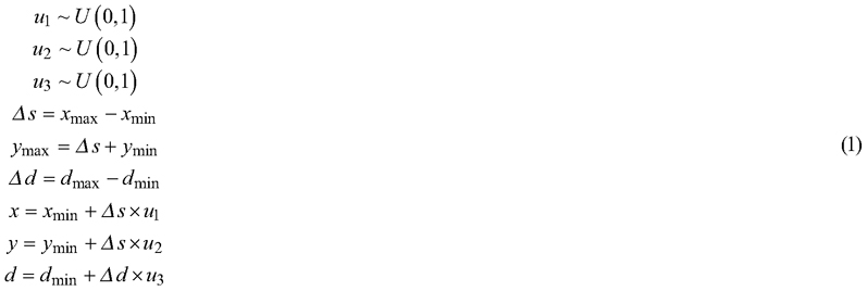
The trees in the simulations were created using a random loop in the python scripting language. Every tree had an x, y coordinate in the plane and a stem diameter d. Coordinates were generated using uniform distributions U, with equal probability between a span of min and max values, Δs = xmin – xmax = ymin – ymax, filling a square (Eq. 1). Stem diameters were randomly generated, using a uniform distribution U, with equal probability between a span of min and max diameters, Δd = dmin – dmax (Eq. 1) The number of generated trees was calculated using the number of stems per hectare value and the selected area in the simulation, rounded to the nearest integer. A new position was randomly generated if there was a neighboring tree within a radius of 1 m, resulting in a minimum tree neighbor distance. The loop ended when the square was filled with the pre-set number of trees. A number of different stem densities were tested in the simulations for areas of a pre-chosen size.
2.2 Simulation of local stem maps with position errors
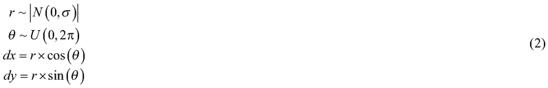
When co-registering a local stem map with a global stem map there may be position differences between the two systems, leading to tree stem linking with errors. To simulate this, a global stem map was created using the method described above. Then a local stem map from the same forest area was generated by cutting a circular plot with a radius of 10 m from the global stem map. A position error (dx,dy) was added to the simulated coordinate for each tree in the local stem map, in order to simulate tree detection sensors with different accuracies. Position errors were modeled as radial displacements r, in random angular directions expressed in radians θ. The radial displacements were modeled as absolute values from a Gaussian distribution with standard deviation σ, and the angular directions were modeled as values from a uniform distribution with the span 0– 2π radians (Eq. 2). The trigonometric functions sin and cos were used to transform values from polar to Cartesian coordinates, (Eq. 2):
A regular stem neighbor distance re was introduced to make it possible to compare simulations with different stem density, ρ (stems m–2) (Eq. 3):

For convenience Eq. 3 is also expressed using the stand density Ρ (stems ha–1), for cases where areas are measured in hectares.
High density stands have a small re, whereas low density stands have a large re. In dense stands there is a higher risk of linking trees incorrectly, and therefore a normalized radial displacement standard deviation, σn, was introduced (Eq. 4) to make it possible to compare sensor errors results from stands with different stem densities:

2.3 Simulation of stem data captured in the path of a moving sensor
A quadratic 100×100 m2 forest stand was generated representing a global stem map, using the method described above. The diameter at breast height span of the trees was set to 0.05–0.30 m and stand density was set to 600 stems ha–1. A moving virtual sensor that sampled trees within this forest stand was then simulated to represent a local stem map. A quadratic sensor path was chosen that started and ended at the same position (0,0), with a side length of 40 m and the speed of the moving sensor set to 1 m s–1. Each simulated detection of a tree was given a sample time along the sensor path for each time step. The sensor path was generated with a sampling interval of 0.1 seconds and the sensor depth of vision was set to 10 m. The sensor path and the depth of vision remained inside the simulated forest stand at all times. For every time step in the sampling interval all visible trees closer than the depth of vision to the sensor were considered ‘detected’ and were saved at that time step and labeled with the corresponding sample time. The trees further away from the sensor and the ones where the view was blocked by another tree in front of them were not included at this time step. It was possible for a tree to be visible in some time steps but shaded in others when the sensor had moved a few more meters.
Sensors producing local stem maps have measurement errors when sampling from forest stands. To simulate a sensor with errors, radial displacements of the simulated detected trees with a standard deviation of 0.25 m was added with the method described above. A drift of 0.050 m s–1 in the x-direction and 0.025 m s–1 in the y-direction was also added to the trees in the path to simulate a sensor with a calibration that is drifting with time. A shift of 3 m in the y-direction was also added to the trees after 100 seconds to simulate a sudden bias of the signal. Two random error trees were added at every time step, and shaded trees were excluded from calculations to simulate omission and commission errors. A plot of this size and density with the chosen configuration would have about 19 trees at every time step, where two are shaded and not visible by the sensor.
In order to simulate an algorithm that samples from several time steps, the algorithm sampling interval was set to be larger than the sampling interval of the sensor path; 0.5 seconds with a 0.25-second duration, covering trees sampled from different times at slightly different positions.
2.4 Stem map co-registration algorithm
The stem map co-registration method is based on the assumption that you have two datasets of single trees that are to be linked and transformed into either of the two coordinate systems. The assumption is that the first dataset is a large global stem map which could be a forest stand or a large field plot. The second dataset is assumed to be a local stem map; for instance, from data registered by a moving sensor. Both datasets should have 2D positions of x, y, for each tree and variables of comparable size; in this study the stem diameter at breast height, d. In the case of a moving sensor, there should also be a sampling time associated with the capture of each tree diameter. In some cases, a moving sensor can have several diameters captured at different height intervals at different times, which is allowed by the algorithm. The assumption is also that datasets have small errors in the z-direction, making it possible to work purely on the x, y coordinate plane. A heavily-inclined tree where the position is determined by the top of the tree rather than the root of the tree will have a position error added to the x, y coordinate of the root position.
2.4.1 Link quality metric by diameter weighted tree neighbor distance
Sometimes small trees are present in one of the datasets but not in the other, which can cause linking errors in the co-registration process if a small tree is located close to a large neighboring tree in the corresponding data set. To avoid this, a diameter-weighted neighbor tree distance rw was introduced that weighs the Euclidean distance, in the 2D xy-plane (rn) by the ratio of the diameters of the neighboring trees; the larger diameter of the two stems, dmax, in the numerator and the smaller diameter of the two stems, dmin, in the denominator (Eq. 5). This gives the Euclidean neighbor distance if the diameters are equal but twice the Euclidean distance if one diameter is two times the size of the other diameter. This means that trees with large diameter differences have a lower probability of being linked, compared to trees where diameters are similar.

For every pair of linked neighbor trees, a quality weight, w, was introduced (Eq. 6). If the distance between the linked trees is zero, the weight (w) is one. If the distance between the trees is large, the weight (w) approaches zero.

2.4.2 Co-registration quality metric and threshold
A co-registration quality metric Q was introduced as the sum of all pair link quality weights (Eq 7), normalized by the number of trees N in the field plot (or in the case of a moving sensor, the number of detected trees within a time period). If all trees are perfectly linked with zero distances the total quality of the co-registration will be one. If some trees have no links or if some trees have position errors, the quality metric Q will be smaller than one and approaching zero for co-registrations that are likely incorrect. A minimum threshold value, QT, for when the quality value Q shows a co-registration that is likely correct needs to be found empirically.

2.4.3 Stem linking algorithm
Before linking two field datasets, the datasets are saved in 10×10 cm quad trees in the x, y-plane for easy access using coordinates. In that way there is no need to search the whole list for every test. Quad trees are data structures that recursively subdivide regions into four at every resolution level, which makes it possible to quickly search and find objects within a selected region (Samet 1984). The quad tree cell that surrounds the investigated coordinate x, y of interest will contain trees of interest or be empty.
If the tree lists (filled-in quad tree cells) already have coordinates that are close both in x, y positions and rotations there is no need to do a massive search of the Euclidean space. The only necessity is linking the separate trees in the datasets. This can, for instance, appear when a previous time step already has co-registered the stem coordinates to be close enough or when two data sources with accurate geographical measurements are used. The co-registration quality metric Q can be used to determine whether a pure linkage is sufficient.
The stem linking algorithm works as follows:
For every tree in the local stem map, find the closest trees within a given search radius R in the corresponding global stem map. Within this search space, find the matching trees with the smallest weighted neighbor distance rw, (Eq 5). Save the chosen tree pair in a dictionary for later access. There might be more than one tree that connects to a particular tree in the global stem map. When all trees are processed, search the found tree pairs for conflicts. If a tree from the global stem map has several trees from the local stem map linked to it, keep the pair with the highest linking quality weight w (Eq 6). In some cases, one wants to keep all field plot trees connected to a forest stand tree; for instance when a moving sensor has several detected diameters at different height levels and different times. In such cases leave all pairs in the list.
2.4.4 Stem map matching algorithm
When tree lists have different coordinate systems and different rotations, for instance at the start of the moving sensor path or after a time step with unsuccessful linking (Q < QT), there is a need to match and find the correct homogeneous transformation that transforms the local stem map coordinates (xl,yl), to global stem map coordinates (xg,yg), where θ is the rotation angle, and tx and ty are the translation.

An appropriate search space in the forest stand is chosen where there is a high probability for the local stem map to be positioned correctly. If an approximate center coordinate is known, the search space can be smaller. Otherwise, the whole global stem map needs to be investigated. A small search resolution incremental distance of ds is chosen, equal in this study to 1 m. The ds value should be small enough to make linking correct trees possible. For dense stands this number must be small. For every x and y coordinate within the search space, the coordinates should be incremented by ds for every step. If the field plot is rotated, several rotations also need to be tested. In this case, the angular step should be small enough to give a maximum arc length of ds at the periphery of the local stem map.
For every coordinate and rotation in the search space, do a stem linkage as described above. Calculate the co-registration quality value Q. Keep the matched tree pair list that gives the highest quality Q. Use the final matched stem pair list to find the transformation parameters θ, tx and ty by minimizing the square of the residuals. Once the parameters are found, the whole dataset can be transformed to either of the two coordinate systems and thus be co-registered.
2.4.5 Moving sensor co-registration algorithm
There needs to be a separate transformation for every time step if one of the datasets is captured by a moving sensor that does not have perfect geographical registration and that may have drift and sudden bias in the process. In this case, the algorithm works on subsets of the MLS data selected at short time spans. The time spans must be long enough to contain several trees in the local neighborhood, but short enough to make the trees appear to be almost standing still in the moving sensor setup. The speed of the moving sensor and the sampling interval of the sensor will offer appropriate values for these parameters.
The algorithm starts by filtering out the sensor-detected trees from the first time span and performs a stem linkage as described above. The linkage is assumed to be correct if the quality Q > QT. If the co-registration quality Q is lower than the threshold there will be a stem map matching of the tree lists as described above. The time, the transformation matrix, and the quality weight Q will be saved in a list if the sampled trees at the time span have produced an acceptable quality Q either by direct linkage or by stem map matching. If not, the previous transformation matrix will be used. The algorithm then continues by filtering out the sensor-detected trees from the next time span and proceed with the iteration. The algorithm stops when there are no more time steps.
The list of homogeneous transformation matrices for each time step and each weight Q are then used to transform the different stems in the tree list for every tree and time step. If a tree has a time stamp that lies between the time stamps of two saved transformation matrices, a linear interpolation of the stem coordinates from the two transformations determines the final position.
2.5 Evaluation of the algorithms
2.5.1 Diameter weighted stem linking accuracy
A simulation with different settings of diameter intervals and stand densities was performed to evaluate the accuracy of the diameter weighted linking algorithm. The chosen diameter intervals were (0.30–0.30 m), (0.15–0.30 m), (0.10–0.30 m), (0.10–0.40 m), (0.10–0.50 m) and (0.10–0.60 m), and the chosen stand densities were 500, 1000 and 1500 stems ha–1. For each setting, 5000 forest stands were simulated, each with a random normalized radial displacement standard deviation position error σn, in the interval 0–2 for the circular field plots. The ratio between the number of correctly linked trees and the total number of trees in each simulated plot was saved.
Statistics describing the linkage accuracy ratios were assembled in bins with size 0.1; each for a specific position error (σn) interval. The average linking accuracy ratio, q, for the settings was modeled with two functions for each setting, where C1, C2, p1 and p2 are parameters and σn is the normalized radial displacement standard deviation.
![]()
![]()
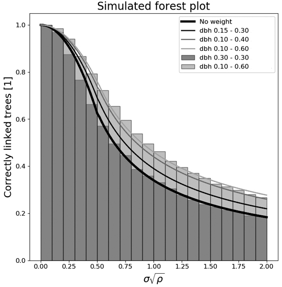
Fig. 1. The number of correctly linked trees in field plots as a function of the normalized radial displacement standard deviation for several different diameter spans of simulated forests. The stand densities used are from an equal amount of 500, 1000, and 1500 stems ha–1.
The inflection point between those two functions was set to a value of σn = 0.5 based on visual inspection of the data, Fig. 1. The value of q = qinf for the inflection point of every setting was linearly interpolated using all σn values between 0.3 and 0.7. Setting the inflection point values in the previous equations gives us:

and

Insert C2 from (Eq. 12) in (Eq. 10):

and divide by qinf :

Linearize using the natural logarithm:

and solve p2 using least squares regression. The parameter p1 is modeled as 2 and C1 and C2 can be extracted from the equations. The parameter settings and the root mean square error of the model fit are shown in the results chapter.
2.5.2 Setting the co-registration quality metric threshold
A quality threshold QT is needed to see whether a field plot co-registration is correct and not just randomly linked trees between similar forest areas. Therefore, a test was performed where 100 pairs of forests stands were simulated for each stand density at 500, 1000, and 1500 stems ha–1. From one of the forest stands a field plot with radius of 10 m was cut out and then matched with the other forest stand. The co-registration quality metric Q was calculated for the matched pair and then saved. Since the pairs were randomly chosen, these quality values should be smaller than would be the case for a correct co-registration. The average and standard deviation of the Q values of the three stand densities were saved.
To obtain a comparison with plots that have correct co-registrations, 100 forest stands for each setting was simulated. The settings were: stand densities 500, 1000, and 1500 stems ha–1, diameter spans 0.3–0.3 m and 0.1–0.6 m and normalized radial displacement standard deviations, σn, of 0.1, 0.2, 0.3 and 0.4. For both simulations the linking tree search radius R was set to 3 m and the search space was set to +/–5 m in the x and y direction.
The co-registration quality threshold QT was manually set to 0.55 m–1 after the simulations of the random and the correct co-registrations were compared, since it resulted in good separation between the two cases. See the results and Fig. 2.
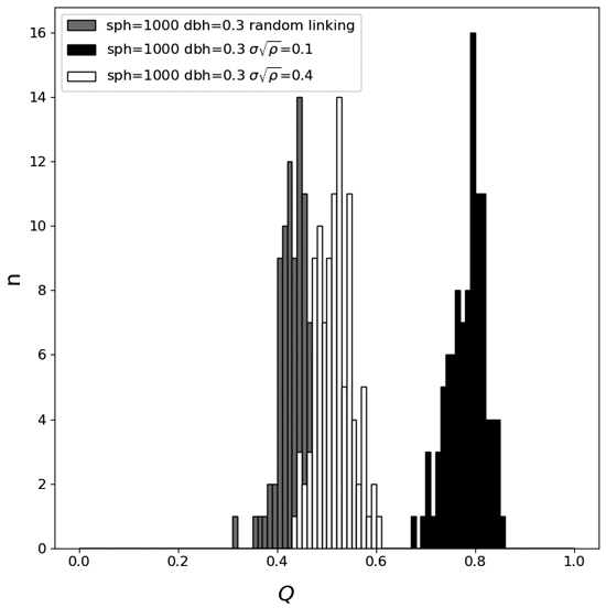
Fig. 2. The co-registration quality metric Q distributions for plots with randomly linked trees and plots with correctly linked trees for two different normalized radial displacement standard deviations. The number of stems ha–1 (sph) was set to 1000 and the diameter at breast height (dbh) was 0.3.
2.5.3 Performance test of co-registration using a moving sensor
As an evaluation of single tree detection with a moving sensor with drift errors, the algorithm was tested on the data from the simulated sensor detection path described above. The number of correctly linked trees was recorded, as was the average link distance and standard deviations of the tree positions after the moving sensor was transformed to the global coordinate system of the forest stand. See the Results and Fig. 3.
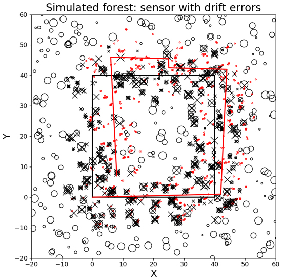
Fig. 3. A simulation of a moving sensor with drift errors co-registering a forest stand. The black circles are trees from the forest stand with diameters proportional to the size of the trees. The black rectangle is the true sensor path, and the red track is the sensor path with errors. The small red dots are the tree positions with errors and the black x’s are the tree positions after co-registration.
2.5.4 Co-registration using real sensor data from a forest stand
The co-registration algorithm was tested with data from an MLS system consisting of a Velodyne VLP 16 laser scanner (Xsense MTi-G-710 inertial navigation system) and a Jetson AXG Xavier computer. An initial point cloud was first derived using LIO-SAM (Shan et al. 2022). The point cloud and sensor trajectory were further calibrated using forest-specific features, as described by Tulldahl et al. (2019), and tree stem positions and stem diameters were derived using the corrected point cloud (Holmgren et al. 2019). A rigid body transformation between local and global coordinates was computed using pairs of coordinates from the calibrated sensor trajectory, where GNSS data were available. The rigid body transformation was then used to transform from local to global tree coordinates, resulting in an initial global tree map from MLS data (Fig. 4). The test site was scanned with the ALS system Leica TerrainMapper, and individual tree crowns were segmented with a system that uses tree crown templates (Holmgren et al. 2022), to produce a global tree map from ALS data containing tree positions, tree heights, and estimated stem diameters. A digital surface model (Fig. 4) was also derived from ALS data for visualization. The algorithm was tested using the global tree maps from MLS and ALS data and used as input to derive a final global MLS tree map (Fig. 4).
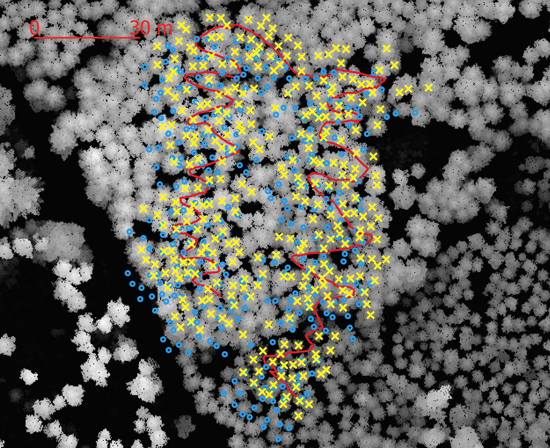
Fig. 4. Co-registration of aerially detected stem positions and ground reference stem positions of a forest stand using the algorithm described in the paper. Blue circles are stem positions before co-registration and yellow x’s are stem positions after co-registration. The red curvy line is the sensor path. The gray background is the canopy height model derived from airborne laser scanner data.
To evaluate the global MLS tree maps before and after co-registration, the shortest horizontal distance λ from each MLS tree position to the nearest ALS tree position was derived for both tree maps. Descriptive statistics of nearest neighbor distances were derived to see how well the stems aligned in the MLS and ALS data. In addition, a visual inspection of the co-registered stem positions and the digital surface model was performed to see how well the stems aligned with the canopy treetops (Fig. 4). The root mean square difference M was introduced as a measure of the dispersion between the two datasets (Eq. 16), where T is the number of observations:

3 Results
3.1 Diameter weighted linking accuracy
The diameter weighted tree stem position linking algorithm works well, as can be seen in Fig. 1 and Table 1 – as long as the detector’s position errors are small. If the normalized radial displacement standard deviation, σn, is smaller than 0.25, the number of correctly linked trees will be higher than 90% for most settings (Table 1). This would mean a radial displacement standard deviation, σ, of 1.12 m for a 500-stem ha–1 stand, 0.79 m for a 1000-stem ha–1 stand, and 0.64 m for a 1500-stem ha–1 stand. In Fig. 1 it can also be seen that the weighted algorithm works better the more diverse tree stem diameters happen to be in a stand. It can also be seen that for homogeneous stands with equal stem diameters, the linking algorithm is equal to a pure Euclidean linking algorithm where the distance to the neighbor tree is the only aspect used.
| Table 1. Number of detected trees [%] at different settings of the span of diameter at breast height and normalized standard deviation of the position error σ√ρ. The average of simulated plots 500, 1000, and 1500 stems per hectare were used. | ||||||
| σ√ρ | Dbh 30 cm | Dbh 15–30 cm | Dbh 10–30 cm | Dbh 10–40 cm | Dbh 10–50 cm | Dbh 10–60 cm |
| 0.05 | 99.9 | 99.9 | 100.0 | 100.0 | 99.9 | 100.0 |
| 0.15 | 96.8 | 98.0 | 98.4 | 98.5 | 98.4 | 98.6 |
| 0.25 | 87.6 | 91.5 | 92.3 | 92.6 | 93.6 | 94.1 |
| 0.35 | 76.6 | 82.6 | 83.9 | 85.5 | 86.0 | 86.7 |
| 0.45 | 66.2 | 72.3 | 75.7 | 76.9 | 77.7 | 79.4 |
| 0.55 | 57.1 | 64.7 | 67.2 | 69.4 | 70.4 | 72.2 |
| 0.65 | 49.6 | 56.2 | 60.4 | 63.4 | 64.5 | 65.5 |
| 0.75 | 44.6 | 51.1 | 53.7 | 56.3 | 58.0 | 59.6 |
| 0.85 | 38.7 | 46.7 | 49.7 | 50.7 | 53.3 | 53.9 |
| 0.95 | 35.9 | 41.4 | 45.4 | 47.4 | 48.6 | 49.6 |
| 1.05 | 33.1 | 38.5 | 41.8 | 43.6 | 45.3 | 46.2 |
| σ = stem position radial displacement standard deviation. ρ = the number of stems m–2. Dbh = diameter at breast height. | ||||||
The parameters of (Eqs. 9 and 10) were curve fitted and saved in Table 2 together with the root mean square error of the model fit, as an overview of how the average linking accuracy ratio, q, depends on the normalized radial displacement standard deviation for different settings of diameter spans and stand densities. A few of those curves are plotted in (Fig. 1). The stand densities used were 500-, 1000-, and 1500-stem ha–1, and the combined results of all three (to be used if the stem density in the stand is non-homogeneous).
| Table 2. Curve fitted function parameters for detection rates in the simulations with different diameter settings at breast height ratio and different numbers of stems per hectare. | |||||||
| Dbh [m] | Dbh ratio | Sph [ha–1] | C1 | p1 | C2 | p2 | Rmse |
| 0.30–0.30 | 1.0 | all | 1.5 | 2.0 | 0.34 | –0.89 | 0.101 |
| 0.30–0.30 | 1.0 | 500 | 1.55 | 2.0 | 0.34 | –0.86 | 0.127 |
| 0.30–0.30 | 1.0 | 1000 | 1.49 | 2.0 | 0.33 | –0.91 | 0.086 |
| 0.30–0.30 | 1.0 | 1500 | 1.47 | 2.0 | 0.34 | –0.9 | 0.081 |
| 0.15–0.30 | 2.0 | all | 1.24 | 2.0 | 0.39 | –0.83 | 0.102 |
| 0.15–0.30 | 2.0 | 500 | 1.29 | 2.0 | 0.39 | –0.8 | 0.132 |
| 0.15–0.30 | 2.0 | 1000 | 1.23 | 2.0 | 0.39 | –0.84 | 0.088 |
| 0.15–0.30 | 2.0 | 1500 | 1.2 | 2.0 | 0.39 | –0.85 | 0.075 |
| 0.10–0.40 | 4.0 | all | 1.05 | 2.0 | 0.44 | –0.76 | 0.099 |
| 0.10–0.40 | 4.0 | 500 | 1.07 | 2.0 | 0.44 | –0.74 | 0.127 |
| 0.10–0.40 | 4.0 | 1000 | 1.05 | 2.0 | 0.43 | –0.76 | 0.089 |
| 0.10–0.40 | 4.0 | 1500 | 1.02 | 2.0 | 0.43 | –0.78 | 0.073 |
| Dbh = diameter at breast height. Sph = stems per hectare. all = an equal amount of 500, 1000 and 1500 Sph. Dbh ratio = the maximum possible Dbh in the span divided by the minimum possible Dbh in the span. Rmse = root mean square error of model fit residuals. | |||||||
For details see Supplementary file S3.
3.2 Setting the co-registration quality metric threshold
Fig. 2 shows the histograms of the co-registration quality metric Q for three different settings. There it can be seen that the co-registration of a stand with small detector position errors is easy to discriminate from a random linkage of two separate stands, whereas if the stand has large detector position errors the distribution is more similar to the random linking distribution. Table 3 shows the average and standard deviation of the co-registration quality metric Q for three different stand densities: 500-, 1000-, and 1500-stem ha–1 for random linking of stands. It is also shown that there is more than a 99% probability that the Q value is smaller than 0.55 for all three stand densities (if the histograms are assumed to be Gaussian), making QT a suitable threshold value. All values smaller than this are probably incorrect stem map matching.
| Table 3. Statistics of the co-registration quality metric Q for different number of stems ha–1 for randomly combined plots. These values are used to set a minimum Q threshold for the level of possible correctly-linked field plots. Values lower than this are probably caused by incorrect co-registrations. | ||||
| Stems ha–1 | avg Q | StdDev Q | Avg + 3 stdDev | Probability Q < 0.55 [%] |
| 500 | 0.416 | 0.0520 | 0.572 | 99.51 |
| 1000 | 0.442 | 0.0372 | 0.553 | 99.82 |
| 1500 | 0.459 | 0.0288 | 0.545 | 99.92 |
| avg = average. StdDev = population standard deviation. | ||||
In Table 4 the results from correctly-linked stands with a different number of settings are shown, and it can be seen that as long as the normalized radial displacement standard deviation of the stem position error is smaller than 0.3, there is a high probability that the co-registration quality metric Q is higher than 0.55, making this a suitable threshold value.
| Table 4. Statistics for the co-registration quality metric Q for different number of stems ha–1, and normalized position error standard deviation σ√ρ, for correctly co-registered plots. Small stem position errors make it easier to separate a correct co-registration from an incorrect one. | |||
| Stems ha–1 | σ√ρ | Dbh [m] | Probability (Q > 0.55) [%] |
| 500 | 0.1 | 0.3–0.3 | 100.0 |
| 500 | 0.1 | 0.1–0.6 | 100.0 |
| 1000 | 0.1 | 0.3–0.3 | 100.0 |
| 1000 | 0.1 | 0.1–0.6 | 100.0 |
| 500 | 0.2 | 0.3–0.3 | 83.53 |
| 500 | 0.2 | 0.1–0.6 | 91.4 |
| 1000 | 0.2 | 0.3–0.3 | 99.06 |
| 1000 | 0.2 | 0.1–0.6 | 99.96 |
| 500 | 0.3 | 0.3–0.3 | 31.36 |
| 500 | 0.3 | 0.1–0.6 | 31.72 |
| 1000 | 0.3 | 0.3–0.3 | 66.78 |
| 1000 | 0.3 | 0.1–0.6 | 79.04 |
| 500 | 0.4 | 0.3–0.3 | 3.93 |
| 500 | 0.4 | 0.1–0.6 | 10.93 |
| 1000 | 0.4 | 0.3–0.3 | 16.82 |
| 1000 | 0.4 | 0.1–0.6 | 27.25 |
| Dbh = the diameter at breast height. σ = stem position radial displacement standard deviation. ρ = the number of stems m–2. | |||
For more details see Suppl. file S3.
3.3 Performance test of co-registration using a moving sensor
When evaluating the performance of the algorithm on the simulated moving sensor in a forest stand, most of the trees where correctly linked at 89.35%, even though the sensor had a drift with time and had different types of positioning errors and omission and commission errors Fig. 3. The average tree link distance was 0.314 m, which was close to the modeled random position error. The standard deviation of the tree link distance was 0.301 m. The co-registration and linking process was completed within 2.65 hours on an Intel®, CoreTM i7CPU 2.30 GHz * 8 with a global stem map of 600 trees and a local stem map sampling of 30 000 tree positions. Note that each stem is scanned from different directions at different times, as the simulated sensor moves along the path resulting in more stem positions in the local stem map than in the global stem map. In Fig. 3 some trees can be seen that do not link to the global stem map. Those trees are either the result of commission errors from the simulated detector or result from errors in co-registration during some of the scan time samplings steps.
3.4 Co-registration using real sensor data from a forest stand
A visual inspection of the stem positions after co-registration show that they align with the canopy height model (Fig. 4) which indicates that the algorithm is functioning as expected. Since the trees were not labeled, it was not possible to evaluate the linkage rate at the single tree level but the MLS-tree to nearest ALS-tree distance decreased after the datasets were co-registered. The average distance decreased from 1.90 to 0.51 m, the standard deviation of the nearest distances decreased from 1.00 to 0.38 m, and the root mean square difference (Eq. 16) of the distances decreased from 2.15 to 0.64 m, which indicates that the datasets are better aligned after co-registration.
4 Discussion
The presented algorithm works when using simulated data from a moving sensor with drift errors, and the accuracy of the method increases in the case of datasets with heterogeneous diameter distributions. In comparison to the study by Hyyppä et al. (2021), which also used simulated data together with three boreal test sites, one can see that the behavior is similar. Their definition of success rate is slightly different than the measurement of correctly linked trees in this paper, but one can see in, for instance, Fig. 6d of their paper that the success rate starts to decline at a standard deviation of 0.5 m. This is also seen in our study. The selected stand density of 750 stems ha–1, in their paper, would give a normalized radial displacement standard deviation of 0.14 (Eq. 4), which indicates the same behavior (Fig. 1 in our paper). Fortunately, many modern single tree detectors have much smaller deviations than 0.5 m. For example, a stem location root mean square error of less than 10 cm in the study by Liang et al. (2018). Fig. 6d in the paper by Hyyppä et al. (2021) also show that the success rate increases when using size descriptors, which is also the case in our study when using the diameter weighted tree neighbor distance (Eq. 5; Fig. 1).
Earlier studies that co-register ALS data with TLS data or manual field-sampled data usually have high success rates. Korpela et al. (2007), for instance, had an observation imprecision of points of about 0.2 m in the X and Y directions, in their semi-manual photogrammetric method, in a 50-year-old pine–spruce–birch test site in Finland. Olofsson et al. (2008) had a of 92.9% proportion of connected trees after co-registering ALS data (10 points m–2) to 155 manually inventoried field plots at a Swedish conifer site, and Hauglin et al. (2014) co-registered ALS data (7.5 points m–2), and TLS plots at the 87% accuracy level for positional errors <1 m. For the CHM-based approaches, Dorigo et al. (2010) had a 68% success rate in automatically co-registering 98 NFI-sample plots in Austria. Pascual et al. (2013) had a RMSE of 0.86 for coordinate differences when comparing their method with an electronic theodolite and Monnet and Mermin (2014) co-registered 91% of the plots within two meters in an uneven-aged coniferous forest using high density ALS data, when at least five of the largest trees were included. Paris et al. (2017) improved the normalized cross correlation similarity measure from 0.65 to 0.73 when comparing scans before and after co-registration of ALS and TLS data, in an oak savanna woodland.
The test case with real sensor data from a forest stand indicates that the algorithm works on an actual forestry application and that it could be a tool when working with multiple remote-sensing datasets in forest environments. However, there are issues that need to be solved before it can be used as a universal tool. The underlying assumption in the co-registration algorithm is that the position of the roots of the trees in the x, y plane is detected with an accuracy good enough to make alignment possible. There are cases where this is difficult. For instance, if one of the remote sensing methods detects the tree top positions rather than the root positions, there will be difficulties if the trees are inclined, giving a position difference of 2–3 m. If all trees are of equal height and are inclined in the same direction, this will cancel out by the co-registration algorithm, but this cannot be assumed in every case: heterogeneously inclined forests will not work. One solution could be to use high density remote sensing data that can detect data at the ground level and thereby detect the position of tree roots, rather than the position of the top of the trees, or maybe detect the direction of a stem and by extrapolation obtain an estimate of the root position.
For the algorithm to work well, the number of omission and commission errors need to be small compared to the number of correctly-detected trees. If there are too many commission errors the plot would look too much like a random plot to offer any useful results. However, with the methods tested by Liang et al. (2018) the mean accuracy was approximately 75% in a single scan setup in a plot of size 32×32 m2. In a smaller plot the numbers would be even better, for instance in Olofsson and Holmgren’s (2016) study, where the overall detection accuracy of a 10 m radius circular plot was 0.9. A careful choice of remote sensing method and plot size would likely solve this issue.
The algorithm was implemented using a scripting language which does not offer short computation times. In an industrial application, this method would probably be implemented using a compiled language and parallel processing. Therefore, the algorithm processing speed could probably be increased substantially when using new hardware and optimized implementations.
The evaluation of the presented co-registration methods on both simulated data and on real sensor data indicates that the algorithms works, and that it could be a valuable tool in forestry. One use case could, for instance, be to use the methods when co-registering harvester data with other remote sensing data.
5 Conclusions
A stem diameter weighted linking algorithm was introduced that improves accuracy when operating on diverse diameter stands when using single tree detectors with stem positioning errors. The amount of correctly linked trees improves from 87.6% to 94.1% when the diameter span of the stand is from 10–60 cm, compared to a stand with uniform stem diameters of 30 cm at the normalized radial displacement standard deviation level 0.25 (Table 1).
A co-registration quality metric was introduced that makes it possible to discriminate with high probability between correct and incorrect stem map co-registrations. A threshold value of QT = 0.55 gives a more than 99% probability of finding incorrect co-registrations. Values lower than the threshold should be discarded. There is a high probability of finding a correct co-registration, as long as the normalized radial displacement standard deviation, σn, of the sensor is lower than 0.3.
A new SLAM based co-registration method for stem maps measured with moving sensors was introduced that operates with a high linking accuracy, which can handle sensors with drifting errors and signal bias. A test with simulated data show that the method resulted in an 89.35% detection rate with a synthetic sensor that had position errors, omission and commission errors, and drift. It was also shown that the mean of the nearest neighbor distances decreased from 1.90 to 0.51 m when testing the method on real sensor data, indicating that datasets are better aligned after co-registration.
Models were curve fitted to the average linking accuracy ratio on the normalized radial displacement standard deviation for different settings of diameter spans and stand densities (Fig. 1; Table 2).
The evaluation of the co-registration methods on both simulated data and on real sensor data indicates that the algorithm works and that it could prove valuable to forestry application.
Declaration of openness of research materials data and code
The algorithms are described and open for anyone to use. The data from randomly simulated forests are different for every simulation and not saved. The results from the statistical investigations and the parameters for the average linking accuracy ratios are published in tables. Python code for linking and generating forests are submitted as Supplementary files S1, S2. Python 3 is an open-source language.
Authors’ contributions
Kenneth Olofsson: methodology, analysis, software, writing
Johan Holmgren: concept, review, and editing
Declaration of interest
The authors declare no conflict of interest.
Funding
This project was funded by Skogens Nya Innovationer (SNI) at Skogstekniska klustret, Skogssällskapet, Carl Tryggers foundation, Brattås foundation, the Mistra digital forest research program, and the Royal Swedish Academy of Agriculture and Forestry (Tandem Forest Values program).
Acknowledgments
We would like to thank the staff at Komatsu Forest R&D in Umeå for help with the concept and testing of the algorithm and the Swedish Defence Research Agency (FOI) for building the MLS system. We would also thank the reviewers for their valuable comments.
References
Dorigo W, Hollaus M, Wagner W, Schadauer K (2010) An application-oriented automated approach for co-registration of forest inventory and airborne laser scanning data. Int J Remote Sens 31: 3135–3149. https://doi.org/10.1080/01431160903380581.
Durrant-Whyte H, Bailey T (2006) Simultaneous localization and mapping: part I. IEEE Robot Autom Mag 13: 99–110. https://doi.org/10.1109/MRA.2006.1638022.
Forsman M, Börlin N, Holmgren J (2016a) Estimation of tree stem attributes using terrestrial photogrammetry with a camera rig. Forests 7, article id 61. https://doi.org/10.3390/f7030061.
Forsman M, Holmgren J, Olofsson K (2016b) Tree stem diameter estimates from mobile laser scanning using line-wise intensity based clustering. Forests 7, article id 206. https://doi.org/10.3390/f7090206.
Hauglin M, Lien V, Næsset E, Gobakken T (2014) Geo-referencing forest field plots by co-registration of terrestrial and airborne laser scanning data. Int J Remote Sens 35: 3135–3149. https://doi.org/10.1080/01431161.2014.903440.
Holmgren J, Tulldahl M, Nordlöf J, Nyström M, Olofsson K, Rydell J, Willén E (2017) Estimation of tree position and stem diameter using simultaneous location and mapping with data from a backpack-mounted laser scanner. Int Arch Photogramm Remote Sens Spatial Inf.Sci XLII-3/W3: 59–63. https://doi.org/10.5194/isprs-archives-XLII-3-W3-59-2017.
Holmgren J, Tulldahl M, Nordlöf J, Willén E, Olsson H (2019) Mobile laser scanning for estimating tree stem diameter using segmentation and tree spine calibration. Remote Sens 11, article id 2781. https://doi.org/10.3390/rs11232781.
Holmgren J, Lindberg E, Olofsson K, Persson H J (2022) Tree crown segmentation in three dimensions using density models derived from airborne laser scanning. Int J Remote Sens 43: 299–329. https://doi.org/10.1080/01431161.2021.2018149.
Hyyppä J, Hyyppä H, Leckie D, Gougeon F, Yu X, Maltamo M (2008) Review of methods of small-footprint airborne laser scanning for extracting forest inventory data in boreal forests. Int J Remote Sens 29: 1339–1366. https://doi.org/10.1080/01431160701736489.
Hyyppä E, Yu X, Kaartinen H, Hakala T, Kukko A, Vastaranta M, Hyyppä J (2020) Comparison of backpack, handheld, under-canopy UAV, and above-canopy UAV laser scanning for field reference data collection in boreal forests. Remote Sens 12, article id 3327. https://doi.org/10.3390/rs12203327.
Hyyppä E, Muhojoki J, Yu X, Kukko A, Kaartinen H, Hyyppä J (2021) Efficient coarse registration method using translation- and rotation-invariant local descriptors towards fully automated forest inventory. ISPRS J Photogramm Remote Sens 2, article id 100007. https://doi.org/10.1016/j.ophoto.2021.100007.
Korpela I, Tuomola T, Välimäki E (2007) Mapping of forest plots: an efficient method combining photogrammetry and field triangulation. Silva Fenn 41: 457–469. https://doi.org/10.14214/sf.283.
Lalonde J-F, Vandapel N, Huber D F, Hebert M (2006) Natural terrain classification using three-dimensional ladar data for ground robot mobility. J Field Robot 23: 839–861. https://doi.org/10.1002/rob.20134.
Liang X, Kankare V, Hyyppä J, Wang Y, Kukko A, Haggrén H, Yu X, Kaartinen H, Jaakkola A, Guan F, Holopainen M, Vastaranta M (2016) Terrestrial laser scanning in forest inventories. ISPRS J Photogramm Remote Sens 115: 63–77. https://doi.org/10.1016/j.isprsjprs.2016.01.006.
Liang X, Hyyppä J, Kaartinen H, Lehtomäki M, Pyörälä J, Pfeifer N, Holopainen M, Brolly G, Francesco P, Hackenberg J, Huang H, Jo H-W, Katoh M, Liu L, Mokroš M, Morel J, Olofsson K, Poveda-Lopez J, Trochta J, Wang D, Wang J, Xi Z, Yang B, Zheng G, Kankare V, Luoma V, Yu X, Chen L, Vastaranta M, Saarinen N, Wang Y (2018) International benchmarking of terrestrial laser scanning approaches for forest inventories. ISPRS J Photogramm Remote Sens 144: 137–179. https://doi.org/10.1016/j.isprsjprs.2018.06.021.
Lindberg E, Holmgren J, Olofsson K, Olsson H (2012) Estimation of stem attributes using a combination of terrestrial and airborne laser scanning. Eur J For Res 131: 1917–1931. https://doi.org/10.1007/s10342-012-0642-5.
Monnet J-M, Mermin É (2014) Cross-correlation of diameter measures for the co-registration of forest inventory plots with airborne laser scanning data. Forests 5: 2307–2326. https://doi.org/10.3390/f5092307.
Noordermer L, Næsset E, Gobakken T (2022) Effects of harvester positioning errors on merchantable timber volume predicted and estimated from airborne laser scanner data in mature Norway spruce forests. Silva Fenn 56, article id 10168. https://doi.org/10.14214/sf.10608.
Olofsson K, Holmgren J (2016) Single tree stem profile detection using terrestrial laser scanner data, flatness saliency features and curvature properties. Forests 7, article id 207. https://doi.org/10.3390/f7090207.
Olofsson K, Lindberg E, Holmgren J (2008) A method for linking field-surveyed and aerial-detected single trees using cross correlation of position images and the optimization of weighted tree list graph. In: Proceedings of SilviLaser, pp 17–19.
Paris C, Kelbe D, van Aardt J, Bruzzone L (2017) A novel automatic method for the fusion of ALS and TLS LiDAR data for robust assessment of tree crown structure. IEEE Trans Geosci and Remote Sens 55: 3679–3693. https://doi.org/10.1109/TGRS.2017.2675963.
Pascual C, Martín-Fernández S, García-Montero L, García-Abril A (2013) Algorithm for improving the co-registration of LiDAR-derived digital canopy height models and field data. Agrofor Syst 87: 967–975. https://doi.org/10.1007/s10457-013-9612-2.
Persson H J, Olofsson K, Holmgren J (2022) Forest Inventory using dense airborne laser scanning. Remote Sens Environ 271, article id 112909. https://doi.org/10.1016/j.rse.2022.112909.
Samet H (1984) The quadtree and related hierarchical data structures. ACM Comput Surv 16: 187–260. https://doi.org/10.1145/356924.356930.
Shan T, Englot B, Meyers D, Wang W, Ratti C, Rus D (2020) Lio-sam: tightly-coupled lidar inertial odometry via smoothing and mapping. In: 2020 IEEE/RSJ international conference on intelligent robots and systems (IROS). https://doi.org/10.48550/arXiv.2007.00258.
Thies M, Pfeifer N, Winterhalder D, Gorte BGH (2004) Three-dimensional reconstruction of stems for assessment of taper, sweep and lean based on laser scanning of standing trees. Scand J For Res 19: 571–581. https://doi.org/10.1080/02827580410019562.
Tulldahl M, Rydell J, Holmgren J, Nordlöf J, Willen E (2019) Lidar based positioning in foreast environments. In: Electro-Optical Remote Sensing XIII Conference, part of SPIE Security + Defence International Symposium, Strasbourg, France. SPIE The International society for optics and photonics. https://doi.org/10.1117/12.2533299.
Wang D, Hollaus M, Puttonen E, Pfeifer N (2016a) Automatic and self-adaptive stem reconstruction in landslide-affected forests. Forests 8, article id 974. https://doi.org/10.3390/rs8120974.
Wang Y, Hyyppä J, Liang X, Kaartinen H, Yu X, Lindberg E, Holmgren J, Qin Y, Mallet C, Ferraz A, Torabzadeh H, Morsdorf F, Zhu L, Liu J, Alho P (2016b) International benchmarking of the individual tree detection methods for modelling 3-D canopy structure for silviculture and forest echology using airborne laser scanning. IEEE Trans Geosci Remote Sens 54: 5011–5026. https://doi.org/10.1109/TGRS.2016.2543225.
Total of 29 references.
