Perttu Anttila  ,
Johannes Ojala,
Teijo Palander,
Kari Väätäinen
,
Johannes Ojala,
Teijo Palander,
Kari Väätäinen
The effect of road characteristics on timber truck driving speed and fuel consumption based on visual interpretation of road database and data from fleet management system
Anttila P., Ojala J., Palander T., Väätäinen K. (2023). The effect of road characteristics on timber truck driving speed and fuel consumption based on visual interpretation of road database and data from fleet management system. Silva Fennica vol. 56 no. 4 article id 10798. https://doi.org/10.14214/sf.10798
Highlights
- Finnish road and pavement classes explain driving speed and fuel consumption of a timber truck
- Other significant explanatory variables include the number of road crossings, season, proportion of distance travelled with a loader, and total laden mass of a truck
- In the future, higher-resolution tracking data is needed to construct generalisable models for 76-tonne vehicles.
Abstract
Road transport produces 90% of greenhouse gas emissions in timber transport in Finland. It is therefore necessary to understand the factors that affect driving speed, fuel consumption, and ultimately, emissions. The objective of this study was to assess the effect of road characteristics on timber truck driving speed and fuel consumption. Data from the fleet management and transport management systems of two timber trucks were collected over a year. A sample of 104 trips was drawn, and the tracking points were overlaid on the road data in a geographical information system. Thereafter, work phases were determined for the points, and they were visually classified into road and pavement classes. Subsequently, the data of 80 trips were utilised in regression analysis to further study the effects of the visually interpreted variables on driving speed and fuel consumption. Fuel consumption was explained by the proportion of forest roads and distance travelled with a loader, and the number of crossings and season when driving without a load. When driving with a load, both asphalt and gravel pavements decreased consumption, in contrast to an unpaved road. Crossings increased fuel consumption, as did the winter and spring months, and the total laden mass of the truck. In conclusion, the study showed that the functional Finnish road and pavement classes can be used to predict driving speed and fuel consumption.
Keywords
fuel consumption;
forest roads;
CAN bus;
forest logistics;
greenhouse gas emissions;
log truck;
road classes
-
Anttila,
Natural Resources Institute Finland (Luke), Latokartanonkaari 9, FI-00790 Helsinki, Finland
 https://orcid.org/0000-0002-6131-392X
E-mail
perttu.anttila@luke.fi
https://orcid.org/0000-0002-6131-392X
E-mail
perttu.anttila@luke.fi
- Ojala, UPM Metsä, Sirkkalantie 13 b, FI-80100 Joensuu, Finland E-mail johannes.ojala@upm.com
-
Palander,
School of Forest Sciences, University of Eastern Finland (UEF), Yliopistokatu 7, FI-80100 Joensuu, Finland
https://orcid.org/0000-0002-9284-5443
E-mail
teijo.s.palander@uef.fi
-
Väätäinen,
Natural Resources Institute Finland (Luke), Yliopistokatu 6, FI-80100 Joensuu, Finland
https://orcid.org/0000-0002-6886-0432
E-mail
kari.vaatainen@luke.fi
Published 5 January 2023
Views 45050
Available at https://doi.org/10.14214/sf.10798 | Download PDF

1 Introduction
Between 58 and 69 million solid cubic metres of timber were harvested annually in Finland in 2016–2020 (Natural Resources Institute Finland 2021). Timber transport by a vehicle combination consisting of a straight truck, a full trailer, and a self-loader (later referred to as a truck) has clearly been dominant over other transport modes, with an approximately 75% share of transported volume (Strandström 2021). Road transport by trucks is therefore responsible for 90% of greenhouse gas emissions in timber transport (Venäläinen et al. 2021). With stricter EU-level greenhouse gas emission reduction targets, a deeper understanding of the factors affecting the driving speed and fuel consumption of timber trucking is indispensable.
Anttila et al. (2022) divided these factors related to the vehicle, driver, and driving environment. For example, maximum engine output, and the number and dimension of tyres are vehicle-dependent factors affecting fuel consumption (Almer 2015; Walnum and Simonsen 2015; Bousonville et al. 2019). Furthermore, a truck’s total mass has a strong effect on fuel consumption (Demir et al. 2014; Almer 2015; Walnum and Simonsen 2015; Svenson and Fjeld 2016; Perrotta et al. 2017; Ghaffariyan et al. 2018; Bousonville et al. 2019). Driver-related factors include the number of brake applications during a period or the proportion of driving time spent running idle (Almer 2015; Walnum and Simonsen 2015).
Road geometry and surface roughness are known to affect both driving speed and fuel consumption (Svenson and Fjeld 2016; Perrotta et al. 2017; Svenson and Fjeld 2017; Bousonville et al. 2019; Anttila et al. 2022). Road databases contain information on road classes or pavement types. The purpose of road classification may be to direct maintenance, but classes are also correlated with speed and consumption (Almer 2015; Devlin et al. 2008; Holzleitner et al. 2011; Bousonville et al. 2019). Lower road or pavement classes are generally associated with narrower, more curvy roads with poor or no pavement, resulting in a slower speed and higher fuel consumption than on higher class roads (Palander et al. 2021). In addition, each crossing means deceleration or stopping, and subsequently, acceleration, causing an increase in consumption.
In the winter, snow and ice on roads decrease driving speed and increase fuel consumption. With decreasing temperature also aerodynamic drag and rolling resistance increase. New, rough tyres are usually changed before winter, while by the end of the next summer rolling resistance of the worn-off tyres is considerably lower. Furthermore, truck tare masses increase due to winter accessories and snow that accumulates on the structures of the truck (Anttila et al. 2020). Average fuel consumption is therefore higher than in the summer. In the spring, the thaw ‒ and increasingly bad weather conditions in the autumn ‒ have the same effect on speed and consumption. Weather variables or season have therefore been used as explanatory variables (Almer 2015; Walnum and Simonsen 2015; Bousonville et al. 2019; Anttila et al. 2022).
Nurminen and Heinonen (2007) created time consumption models for trucking activities in Finland. They employed a time study for eight 60-t trucks. Separate models were made for each work phase. However, in two example transport cases, the high-end estimate of the 95% confidence interval was twice the low-end estimate, indicating that considerable variation remains that cannot be explained by work phase and transport distance alone. Later, Anttila et al. (2022) tested several explanatory variables to explain timber truck fuel consumption. The study utilised data from a timber truck fleet management system (FMS) combined with road and weather data. Unfortunately, based on the available data, it was impossible to automatically identify individual trips or separate work phases.
This study’s objective was to assess the effect of road characteristics on timber truck driving speed and fuel consumption. In particular, the aim was to assess if the Finnish road functional and pavement classes could be used to predict speed and consumption by work phase. The study is based on a Master’s thesis (Ojala 2021).
2 Materials and methods
The assessment was based on visual interpretation of a road database and data from a fleet management system for 68-t and 76-t timber trucks (Fig. 1). Data about 13 timber trucks were collected between April 2018 and May 2019 (Anttila et al. 2022). During the follow-up period, the odometer reading, cumulative fuel consumption, coordinates, and timestamp were recorded at approximately 10-minute intervals, except for one truck, which had an interval of approximately 1 minute. All the Scania trucks were equipped with factory-installed hardware that collects data from vehicles’ controller area network (CAN) bus. The tracking data were retrieved via the REST interface from Scania FMS, which was operative in all the trucks. For this study, two of the trucks were selected for further examination (Table 1). One of the trucks had a maximum gross vehicle mass (GVM) of 68 tonnes (later referred to as Truck68t) and the other 76 tonnes (Truck76t).
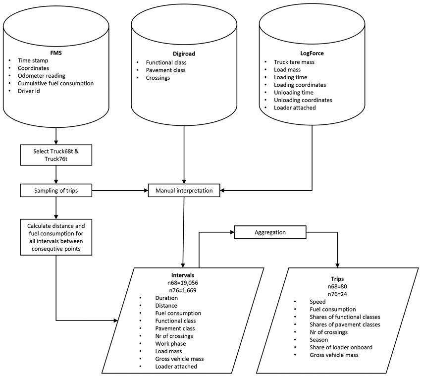
Fig. 1. The procedure to collect trip-level data for modelling of speed and fuel consumption of timber trucks. FMS is the database of a fleet management system, Digiroad the national street and road database, and LogForce the database of a transport management system. The relevant attributes are listed. Truck68t refers to the 68-tonne truck and Truck76t to the 76-tonne truck. n68 and n76 refer to the number of observations of the corresponding trucks.
| Table 1. Basic information of the timber trucks. The notation “*4” indicates the second steered axle was located behind the driven tandem. | |||||||||||
| Combination vehicle | Straight truck | Full trailer | |||||||||
| Id | Gross vehicle mass (t) | Nominal tracking interval (min) | Brand and model | Axle configuration | Commissioned in | Engine displacement (cm3) | Output (kW) | Tare mass (kg) | Loader mass (kg) | Brand and model | Tare mass (kg) |
| Truck68t | 68 | 1 | Scania R 560 | 6×4 | 2013 | 15 607 | 412 | 11 750 | 3500 | Feber Intercars 42P0D6 | 8250 |
| Truck76t | 76 | 10 | Scania R 580 | 8×4*4 | 2017 | 16 353 | 427 | 13 100 | 3800 | Närko D4HS11T11 | 8500 |
To overcome the difficulties of automatically identifying individual trips (Anttila et al. 2022), the road attributes for the FMS data were visually interpreted in a geographical information system (GIS). All the interpretations and spatial analyses were conducted with ArcGIS Desktop 10.6.1 (ESRI 2022). First, a sample of 24 trips for both trucks was drawn from the year-round tracking data. The data were stratified into four three-month periods to ensure the trips covered different weather conditions throughout the year. Subsequently, six trips were randomly sampled from the data of each period.
A trip was assumed to start when an empty truck left a mill and to end when the truck had finished unloading at a destination. To compile a trip, a randomly sampled data point was visually located in the GIS, and the point’s predecessors were tracked until the starting point of the trip was found, and successors until the endpoint was found.
Next, load data were added to the trip. The data were obtained from the LogForce transport management system (Trimble 2021). The data included, inter alia, trucks’ tare masses, load masses based on crane-scale measurements, loading and unloading times and coordinates, and information about whether a loader was attached. With the aid of these data, the work phase and truck’s total mass could be determined for each tracking point (Table 2, Fig. 2).
| Table 2. Work phase division of timber trucking for the estimation of truck speed and fuel consumption (adapted from Nurminen and Heinonen 2007). | |
| Work phase | Definition |
| Driving without load | Begins when the truck leaves the mill storage area after unloading and ends when the truck stops at a roadside storage to receive a new load. |
| Loading | Begins when the truck stops at a roadside storage and ends when the truck leaves for the mill or for travel to the next roadside storage. In addition to actual loading, includes auxiliary activities like preparing the crane, driving between piles, handling the trailer and bunks, and binding the load. |
| Driving between roadside storages | Begins when the truck leaves one roadside storage and ends when the truck stops at the next. |
| Driving with load | Begins when the truck leaves the last roadside storage and ends when the truck stops at a mill yard. |
| Unloading | Begins when the truck arrives at a mill yard and ends when the truck leaves without a load. In addition to actual unloading, includes queueing and waiting, and auxiliary activities like preparations, scaling, and driving between unloading locations. |
| Other driving | Begins when the truck turns off the route and ends when the truck is back on the route. The minimum time for other driving was set at 2 h. |
| Break, max 15 min | Begins when the truck stops for a break of at most 15 minutes and ends when the truck continues driving. |
| Break, over 15 min | Begins when the truck stops for a break of more than 15 minutes and ends when the truck continues driving. |
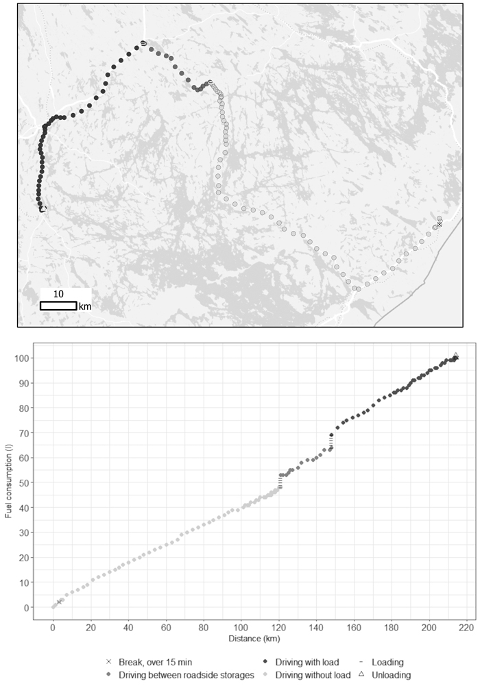
Fig. 2. An example of the interpreted work phases of a trip (above) and the corresponding fuel consumption as a function of driving distance of a timber truck (below).
Road characteristics were based on the DigiRoad national road and street database (Finnish Transport Infrastructure Agency 2018). The database contains the geometry and attribute data of the Finnish road and street network, and it is maintained by the Finnish Transport Infrastructure Agency. In this study, road functional class, pavement class, and the number of crossings were visually interpreted for each road segment between two tracking points by overlaying the points on the road data. To facilitate interpretation, road and pavement classes in the road database were presented with different colours in GIS. Subsequently, the manually identified functional and pavement class and number of crossings were saved with the corresponding road segment data.
The functional class categorises the roads based on the importance of a road for traffic (Finnish Transport Infrastructure Agency 2018). The classes in this study are presented in Table 3. Furthermore, information on road pavement was available in classes presented in Table 4.
| Table 3. Road classes in Digiroad (Finnish Transport Infrastructure Agency 2018) and their reclassification for regression analysis of driving speed and fuel consumption. | |
| Road class | Reclassification |
| Class I main road | Main road |
| Class II main road | Main road |
| Regional road | Main road |
| Connecting road | Collector road |
| Class I private road | Collector road |
| Unknown road class | Collector road |
| Class II private road | Forest road |
| Vehicle track | Forest road |
| N/A | Forest road |
| Table 4. Pavement classes in Digiroad (Finnish Transport Infrastructure Agency 2018) and their reclassification for regression analysis of driving speed and fuel consumption. | |
| Pavement class | Reclassification |
| Hard asphalt concrete | Asphalt |
| Soft asphalt concrete | Asphalt |
| Gravel surface | Gravel |
| Gravel wear layer | Gravel |
| Paved, type unknown | Gravel |
| No pavement | No pavement |
The Google Maps Street View service was utilised for auxiliary information in the interpretation. For each road segment between two tracking points, the work phase, road class, and pavement class covering the longest distance in the segment were selected.
Having collected the first 24 trips for both trucks, it was decided to concentrate further efforts on Truck68t because of the higher temporal resolution of the tracking data. Another 56 trips were therefore interpreted for Truck68t.
Subsequently, a multiple linear regression model was fitted for each of the following dependent variables: 1) speed when driving without a load; 2) speed when driving with a load; 3) fuel consumption when driving without a load; and 4) fuel consumption when driving with a load (Eq. 1).
![]()
where Y = dependent variable, X = explanatory variables, β = model parameters, and ε = error term. The initial explanatory variables included the proportions of the road classes, proportions of the pavement classes, number of road crossings, season, proportion of distance travelled with a loader, and the truck’s total laden mass. The original road and pavement classes were reclassified to reduce multicollinearity (Table 3, Table 4).
One trip was removed from models 1 and 3 because the distance driven without a load was exceptionally short. The models were fitted with a backward stepwise method in IBM SPSS Statistics 27.0.1 (IBM 2021). Residual normality was checked with histograms and homoscedasticity with residual plots.
3 Results
The examined trips of Truck68t and Truck76t totalled 16 209 and 3842 km respectively (Table 5). Nearly half the distance driven by Truck68t was with a load, slightly less (46%) was without a load, and approximately 4% was between roadside storages (Fig. 3). Unlike Truck68t, Truck76t was driving more without than with a load. It was also driving more between roadside storages than Truck68t.
| Table 5. Summary of the examined trips for the 68-tonne and 76-tonne trucks. | ||
| Truck68t | Truck76t | |
| Number of trips | 80 | 24 |
| Average trip distance (km) | 203 | 160 |
| Minimum trip distance (km) | 23 | 60 |
| Maximum trip distance (km) | 385 | 335 |
| Average load (t) | 49.5 | 49.3 |
| Minimum load (t) | 35 | 36.1 |
| Maximum load (t) | 54.1 | 57.7 |
| Number of crossings | 1888 | 490 |
| Total time consumption (h) | 578 | 135 |
| Total fuel consumption (l) | 9279 | 2546 |
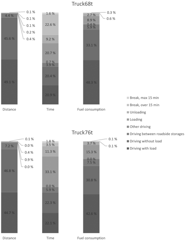
Fig. 3. Distribution of driving distance, driving time, and fuel consumption for the 68-tonne and 76-tonne timber trucks.
The time consumption of timber transport was more evenly divided in work phases than driving distance (Fig. 3). For Truck68t, the proportion of breaks longer than 15 min was about a quarter, whereas driving with and without a load and loading all took one fifth of the time. In the case of Truck76t, significantly more time was spent on loading. Again, for fuel consumption – as with driving distance – the proportion of driving with a load constituted nearly 50% of fuel consumption of Truck68t, whereas for Truck76t, the proportion was slightly lower.
The average trips of Truck68t were longer than the trips of Truck76t: 203 vs. 160 km respectively. The average speed over the whole data was 69 km h–1 for Truck68t and 63 km h–1 for Truck76t. The highest speeds at trip level were reached when driving with or without a load (Fig. 4). In contrast, the average speeds when driving between roadside storages were low: an average of only approximately 30 km h–1.
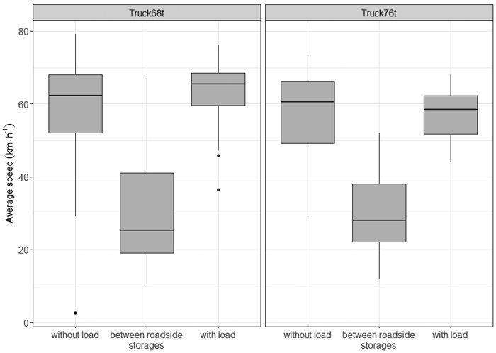
Fig. 4. Distribution of trip-level average truck speed of driving work phases for the 68-tonne and 76-tonne timber trucks.
The average fuel consumption of the lighter truck (Truck68t, 50 l(100 km)–1) was lower than the consumption of the heavier truck (Truck76t, 54 l(100 km)–1) when driving. Loading, unloading and idling increased the total fuel consumption to 57 l(100 km)–1 and 66 l(100 km)–1 respectively. Furthermore, the consumption per tonne kilometre was lower for Truck68t than for Truck76t: 0.012 and 0.013 l(t km)–1. This can be explained by the overweight of Truck68t: the average mass when loaded was 71.6 t for Truck68t and 74.7 t for Truck76t. Average fuel consumption was lowest when driving without a load (43 and 45 l(100 km)–1 for Truck68t and Truck76t), higher when driving with a load (58 and 64 l(100 km)–1), and highest when driving between roadside storages (83 and 76 l(100 km)–1) (Fig. 5). The higher fuel consumption when driving between storages can be attributed to higher share of forest roads. Furthermore, the variance of trip-level fuel consumption when driving between roadside storages was very high, especially for Truck68t. This was due to the fact that the shares of road classes varied considerably more when driving between storages than when driving with or without a load.
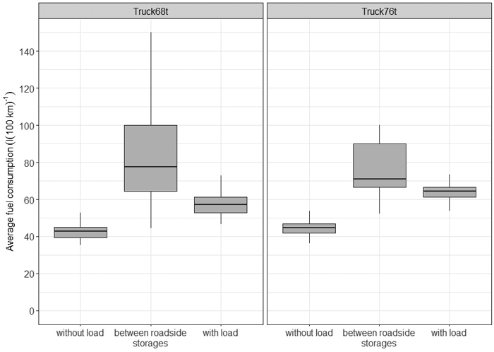
Fig. 5. Distribution of trip-level fuel consumption of driving work phases for the 68-tonne and 76-tonne timber trucks.
In the non-driving work phases, the loading fuel consumption was higher than the unloading consumption (Fig. 6). The average consumption of the former was 7 and 9 l h–1 (0.113 and 0.170 l t–1), and of the latter 5 and 6 l h–1 (0.036 and 0.046 l t–1) for Truck68t and Truck76t.
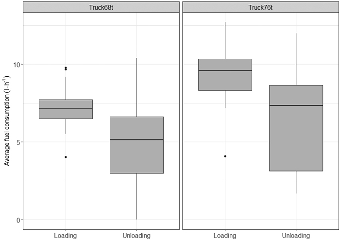
Fig. 6. Distribution of trip-level fuel consumption of non-driving work phases for the 68-tonne and 76-tonne timber trucks.
Most of the trip distances were driven on higher class roads (Table 6). These were mainly paved with hard asphalt concrete. Indeed, the two main road classes with a hard asphalt pavement covered 75% of both trucks’ trips.
| Table 6. Total distances (km) in functional and pavement classes for the 68-tonne and 76-tonne trucks. | ||||||||
| Hard asphalt concrete | Soft asphalt concrete | Gravel surface | Gravel wear layer | Paved, type unknown | Unpaved | Total | ||
| Truck68t | Class I main road | 9465 | 0 | 0 | 0 | 11 | 0 | 9476 |
| Class II main road | 2567 | 857 | 0 | 0 | 0 | 2 | 3426 | |
| Regional road | 258 | 494 | 0 | 0 | 50 | 0 | 802 | |
| Connecting road | 108 | 723 | 8 | 568 | 146 | 2 | 1555 | |
| Class I private road | 1 | 0 | 0 | 0 | 29 | 0 | 30 | |
| Class II private road | 0 | 0 | 0 | 3 | 72 | 745 | 820 | |
| Vehicle track | 0 | 0 | 0 | 0 | 0 | 12 | 12 | |
| No data | 0 | 0 | 0 | 0 | 2 | 10 | 12 | |
| Total | 12 399 | 2074 | 8 | 571 | 310 | 771 | 16 133 | |
| Truck76t | Class I main road | 1368 | 0 | 0 | 0 | 0 | 0 | 1368 |
| Class II main road | 1493 | 0 | 0 | 0 | 0 | 0 | 1493 | |
| Regional road | 337 | 89 | 0 | 0 | 0 | 0 | 426 | |
| Connecting road | 25 | 182 | 0 | 59 | 82 | 0 | 348 | |
| Class I private road | 0 | 0 | 0 | 0 | 17 | 7 | 24 | |
| Class II private road | 0 | 0 | 0 | 0 | 0 | 105 | 105 | |
| Vehicle track | 0 | 0 | 0 | 0 | 0 | 19 | 19 | |
| No data | 0 | 0 | 0 | 0 | 0 | 7 | 7 | |
| Total | 3223 | 271 | 0 | 59 | 99 | 138 | 3790 | |
The highest average truck speeds occurred when driving on main roads (Table 7). One must be cautious when interpreting class-wise speeds. For example, the average speed for Truck68t on class II private road with gravel wear layer was exceptionally high, but the distance in this class was only 3 km. For comparison, the speed values used by ESRI Finland (2019) are given in Table 7. ESRI Finland provides a refined road data set based on Digiroad where time to travel over a road element is calculated from the speed limit of the element. In case the speed limit is missing, the values presented in Table 7 are used.
| Table 7. Average speed (km h–1) in functional and pavement classes for the 68-tonne and 76-tonne trucks. For comparison, the values in ESRI Finland’s (2019) data set are given. The darkness of cell shading indicates speed. | |||||||||
| Hard asphalt concrete | Soft asphalt concrete | Gravel surface | Gravel wear layer | Paved, type unknown | Unpaved | Average | ESRI Finland | ||
| Truck68t | Class I main road | 76 | 40 | 76 | 80 | ||||
| Class II main road | 76 | 71 | 75 | 76 | |||||
| Regional road | 51 | 70 | 28 | 58 | 65 | ||||
| Connecting road | 35 | 52 | 48 | 45 | 33 | 40 | 45 | 48 | |
| Class I private road | 10 | 10 | 40 | ||||||
| Class II private road | 60 | 32 | 20 | 21 | 30 | ||||
| Vehicle track | 9 | 9 | 20 | ||||||
| No data | 4 | 4 | |||||||
| Average | 74 | 63 | 48 | 45 | 26 | 19 | 61 | ||
| Truck76t | Class I main road | 69 | 69 | 80 | |||||
| Class II main road | 70 | 70 | 76 | ||||||
| Regional road | 60 | 46 | 56 | 65 | |||||
| Connecting road | 38 | 45 | 40 | 28 | 38 | 48 | |||
| Class I private road | 15 | 12 | 40 | ||||||
| Class II private road | 17 | 17 | 30 | ||||||
| Vehicle track | 10 | 10 | 20 | ||||||
| No data | 13 | 13 | |||||||
| Average | 68 | 46 | 40 | 24 | 14 | 56 | |||
The road and pavement classes with the highest driving speeds also present the lowest fuel consumptions (Table 8). The highest consumptions were found on vehicle tracks.
| Table 8. Average fuel consumption (l(100 km)–1) in functional and pavement classes for the 68-tonne and 76-tonne trucks. The darkness of cell shading indicates fuel consumption. | ||||||||
| Hard asphalt concrete | Soft asphalt concrete | Gravel surface | Gravel wear layer | Paved, type unknown | Unpaved | Average | ||
| Truck68t | Class I main road | 47 | 82 | 47 | ||||
| Class II main road | 48 | 48 | 48 | |||||
| Regional road | 49 | 47 | 54 | 48 | ||||
| Connecting road | 58 | 54 | 88 | 63 | 59 | 50 | 59 | |
| Class I private road | 62 | 62 | ||||||
| Class II private road | 67 | 67 | 82 | 81 | ||||
| Vehicle track | 133 | 133 | ||||||
| No data | 90 | 81 | ||||||
| Average | 48 | 50 | 88 | 63 | 62 | 83 | 50 | |
| Truck76t | Class I main road | 51 | 51 | |||||
| Class II main road | 53 | 53 | ||||||
| Regional road | 58 | 52 | 57 | |||||
| Connecting road | 60 | 59 | 58 | 59 | 59 | |||
| Class I private road | 82 | 61 | ||||||
| Class II private road | 83 | 83 | ||||||
| Vehicle track | 111 | 111 | ||||||
| No data | 86 | 86 | ||||||
| Average | 52 | 57 | 58 | 64 | 84 | 54 | ||
Truck68t had altogether five and Truck76t eight different drivers in the dataset (Table 9). All the drivers had over three years’ driving experience and had participated in economical driving training. The drivers had distinct distributions of road classes and the distance driven by some of drivers was very short. Therefore, a meaningful comparison of driving speeds and fuel consumptions by driver and road class was possible between drivers 1–3 and 6–7, and for the Class I and II main roads only. With respect to average driving speed the difference between the drivers was 0.3–1.0 km h–1 for Truck68t and 0.1 km h–1 for Truck76t. For average fuel consumption the corresponding differences were 2.4–5.9 l(100 km)–1 and 3.9 l(100 km)–1.
| Table 9. Total driven kilometres by driver for the 68-tonne and 76-tonne timber trucks. | ||
| Truck | Driver | Total distance (km) |
| Truck68t | 1 | 7430 |
| Truck68t | 2 | 6829 |
| Truck68t | 3 | 1362 |
| Truck68t | 4 | 490 |
| Truck68t | 5 | 2 |
| Truck76t | 6 | 1900 |
| Truck76t | 7 | 1371 |
| Truck76t | 8 | 243 |
| Truck76t | 9 | 99 |
| Truck76t | 10 | 90 |
| Truck76t | 11 | 46 |
| Truck76t | 12 | 25 |
| Truck76t | 13 | 9 |
The road and pavement type classes, the number of crossings, and the season explained 84% of the variation in speed when driving without a load and 77% when driving with a load (Tables 10–12). Forest roads, a gravel pavement, and crossings decreased driving speed, whereas an asphalt pavement increased it. Moreover, speed was lower in the winter–spring months and in the autumn when driving with a load.
| Table 10. Statistics of the trip-level speed and fuel consumption models for a 68-tonne timber truck. The unit of RMSE of the speed models is km h–1 and of the fuel consumption models l(100 km)–1. | ||||
| Model | n | RMSE | R2adj | F-test |
| Speed when driving without load | 79 | 4.3 | 0.84 | F(5,73) = 80.47, p < 0.001 |
| Speed when driving with load | 80 | 3.7 | 0.77 | F(6,73) = 43.96, p < 0.001 |
| Fuel consumption when driving without load | 79 | 2.6 | 0.52 | F(5,73) = 18.21, p < 0.001 |
| Fuel consumption when driving with load | 80 | 4.4 | 0.47 | F(6,73) = 12.71, p < 0.001 |
| Table 11. Parameter estimates and test statistics of the 68-tonne timber truck speed models for driving without a load. ForestRoad = proportion of forest roads when driving without a load; Gravel = proportion of poor asphalt and gravel roads when driving without a load; Crossings = number of road crossings when driving without a load ((100 km)–1); DecFeb = 1 if the transport date is within range [December, February], otherwise 0; MarMay = 1 if the transport date is within range [March, May], otherwise 0. | |||
| Term | Estimate | Std. error | t-test |
| Intercept | 77.3 | 1.1 | t(73) = 71.25, p < 0.001 |
| ForestRoad | –44.6 | 5.3 | t(73) = –8.44, p < 0.001 |
| Gravel | –31.4 | 7.4 | t(73) = –4.22, p < 0.001 |
| Crossings | –0.7 | 0.1 | t(73) = –12.51, p < 0.001 |
| DecFeb | –3.1 | 1.2 | t(73) = –2.56, p = 0.013 |
| MarMay | –3.4 | 1.2 | t(73) = –2.81, p = 0.006 |
| Table 12. Parameter estimates and test statistics of the 68-tonne timber truck speed models for driving with a load. ForestRoad = proportion of forest roads when driving with a load; Asphalt = proportion of hard and soft asphalt concrete when driving with a load; Crossings = number of road crossings when driving with a load ((100 km)–1); SepNov = 1 if the transport date is within range [September, November], otherwise 0; DecFeb = 1 if the transport date is within range [December, February], otherwise 0; MarMay = 1 if the transport date is within range [March, May], otherwise 0. | |||
| Term | Estimate | Std. error | t-test |
| Intercept | 36.0 | 6.3 | t(73) = 5.74, p < 0.001 |
| ForestRoad | –22.6 | 13.4 | t(73) = –1.69, p = 0.095 |
| Asphalt | 42.1 | 6.4 | t(73) = 6.57, p < 0.001 |
| Crossings | –0.8 | 0.1 | t(73) = –8.65, p < 0.001 |
| SepNov | –3.2 | 1.2 | t(73) = –2.67, p = 0.009 |
| DecFeb | –2.7 | 1.2 | t(73) = –2.26, p = 0.027 |
| MarMay | –2.8 | 1.2 | t(73) = –2.33, p = 0.023 |
Fuel consumption was explained by the proportion of forest roads, the proportion of the distance travelled with a loader, the number of crossings, and the season when driving without a load (Table 13). These variables could predict more than half the variation in consumption (Table 10). All the explanatory variables increased fuel consumption except for the September–November period.
| Table 13. Parameter estimates and test statistics of the 68-tonne timber truck fuel consumption models for driving without a load. ForestRoad = proportion of forest roads when driving without load; Loader = proportion of distance traveled with a loader when driving without load; Crossings = number of road crossings when driving without load ((100 km)–1); SepNov = 1 if the transport date is within range [September, November], otherwise 0; DecFeb = 1 if the transport date is within range [December, February], otherwise 0. | |||
| Term | Estimate | Std. error | t-test |
| Intercept | 38.0 | 0.9 | t(73) = 40.60, p < 0.001 |
| ForestRoad | 9.0 | 3.2 | t(73) = 2.83, p = 0.006 |
| Loader | 2.5 | 1.0 | t(73) = 2.38, p = 0.002 |
| Crossings | 0.1 | 0.0 | t(73) = 4.17, p < 0.001 |
| SepNov | –3.1 | 0.8 | t(73) = –4.15, p < 0.001 |
| DecFeb | 2.3 | 0.8 | t(73) = 3.074, p = 0.003 |
When driving with a load, the fuel consumption model explained slightly less than half the variation (Table 10). Both asphalt and gravel pavements decreased consumption (Table 14). Again, crossings increased fuel consumption, as did the winter and spring months, and the total laden mass of the truck. The slightly non-linear relationship between mass and consumption was linearised by raising the mass to a power of 1.1.
| Table 14. Parameter estimates and test statistics of the 68-tonne timber truck fuel consumption models for driving with a load. Asphalt = proportion of hard and soft asphalt concrete when driving with a load; Gravel = proportion of poor asphalt and gravel roads when driving with a load; Crossings = number of road crossings when driving with a load ((100 km)–1); Mass = Total mass of the truck (t); DecFeb = 1 if the transport date is within range [December, February], otherwise 0; MarMay = 1 if the transport date is within range [March, May], otherwise 0. | |||
| Term | Estimate | Std. error | t-test |
| Intercept | 86.7 | 17.4 | t(73) = 4.97, p < 0.001 |
| Asphalt | –54.1 | 12.7 | t(73) = –4.25, p < 0.001 |
| Gravel | –44.1 | 15.8 | t(73) = –2.80, p = 0.007 |
| Crossings | 0.4 | 0.1 | t(73) = 3.36, p = 0.001 |
| Mass1.1 | 0.2 | 0.1 | t(73) = 1.75, p = 0.084 |
| DecFeb | 2.9 | 1.2 | t(73) = 2.31, p = 0.023 |
| MarMay | 2.7 | 1.2 | t(73) = 2.26, p < 0.027 |
4 Discussion
Visual interpretation proved a feasible method to collect trip-level data in this study. In manual work, there is always a risk of misinterpretation, but care was taken to minimise it. Once the GIS environment was set, the approximate time consumption for interpreting one trip was 1–2 h, depending on trip length and complexity.
The study shed light on the breakdown to work phases of timber trucking in Finland. Compared to the results on time distribution by Nurminen and Heinonen (2007), the proportions of driving without a load and loading were somewhat higher, whereas the proportions of driving with a load, driving between roadside storages, unloading, and other driving were considerably lower. The proportion of breaks of more than 15 min was remarkably high for Truck68t. The differences may be explained by differences in the operating environment, and – regarding the long breaks – by the fact that due to the definition of a trip, overnight stays could be included in a trip. Furthermore, this study presented distributions of distance and fuel consumption.
As Anttila et al. (2022) stated, the data from the fleet management system had a low resolution of distance and fuel consumption for research purposes. In this study, the effect of these was probably rather small, because the modelling was done at trip level, and the data were collected at a 1-minute nominal interval. Nevertheless, the interpretation method of the share of road and pavement classes may underestimate speed and overestimate fuel consumption on main roads: when interpreting road segments where the road functional or pavement class changed, the class with a longer distance in the segment was selected. The probability of selecting a class therefore increased with increased driving speed. However, in the whole data set the effect is believed to be rather small: when the segments where road or pavement class changed were removed, average speed increased by 5% and fuel consumption decreased by 1%.
When compared with the data of a proprietary product (ESRI Finland 2019), one can see that the average speeds in this study are lower. The difference is especially notable on road classes where the total distance was low, i.e., Class I private road and Vehicle track (Tables 6 and 7). The difference may partly be attributed to the interpretation method. However, the estimation method or accuracy of ESRI Finland’s (2019) data is not known.
Several studies have shown that the fuel consumption obtained from a vehicle’s CAN bus may be inaccurate (Surcel and Michaelsen 2009; Asmoarp et al. 2015; Pink et al. 2017; Venäläinen and Poikela 2020). Furthermore, the results are based on the data of only two trucks, and the alignment of axles or other vehicle deficiencies were not checked during the study by the researchers. Care should therefore be taken, especially when generalising absolute fuel consumption.
The fuel consumption of Truck68t and Truck76t differed little. This can partly be attributed to the overweight of the former. Generally, the fuel consumption of heavier trucks might increase more on forest roads than the consumption of lighter trucks. Lower-level roads imply more decelerations and accelerations than higher-level roads, and accelerating with a heavier mass takes more energy than accelerating with a lighter mass. Since the beginning of this millennium, the maximum GVM has increased in Finland and Sweden (Väätäinen et al. 2021). The increase has been partly motivated by lowering emissions. It is therefore important that the climate benefits of increased masses are not lost in weak road conditions (cf. Palander et al. 2021).
Notwithstanding the inaccuracy of fuel consumption in FMS data, the regression models should represent the effects of the explanatory variables well, as the trends of one truck between trips should be comparable (Pink et al. 2017). The adjusted coefficient of determination was surprisingly high for the speed models and moderate for the consumption models (Table 10). The effects of all the explanatory variables were logical except for SepNov (a binary variable indicating whether the transport date is within range [September, November]) in the model for fuel consumption when driving without a load (Table 13). Basically, this period should not be especially favourable for low fuel consumption. There were only 20 trips in each period, so it is possible that by chance trips with low consumption were selected.
As expected, the effect of road crossings on both speed and consumption was stronger when driving with a load than without a load. Truck mass was not a very strong explanatory variable for fuel consumption when driving with a load. The reason for this may lie in the narrow range of masses in the collected and analysed data (56–78 t).
In addition to the variables included in the models a driver probably also has an effect – especially on fuel consumption. However, due to relatively small dataset it was decided to drop driver effect from the models.
Comparing the models of driving speed with the results by Svenson and Fjeld (2017) reveal that the adjusted coefficients of determination (R2) were approximately at the same level: 84% (without load) and 77% (with load) vs. 65–87% depending on road section length. When it comes to the models of fuel consumption, the values of R2 in this study were somewhat lower than the ones reported by Svenson and Fjeld (2016): 52% (without load) and 47% (with load) vs. 61–85%. The difference could be partly explained by the controlled experiment by Svenson and Fjeld (2016, 2017) and the more detailed explanatory variables like road gradient, curvature, and surface roughness.
Anttila et al. (2022) modelled fuel consumption when driving with load. With their model which used transport distance as the sole explanatory variable the root mean squared error was 9.9 l(100 km)–1 (4.4 l(100 km)–1 in this study). Therefore, the variables in this study clearly explain more of the variation in fuel consumption than the transport distance only.
The explanatory variables could be automatically extracted from road databases and transport management systems, which would enable the utilisation of the models in practice. Additional variables such as road gradient and curvature could still improve the models (Svenson and Fjeld 2016; Svenson and Fjeld 2017; Anttila et al. 2022).
Palander et al. (2020) presented transportation data of 210 trucks operating between 6 July 2018 and 19 August 2020. In their study the average fuel consumption was 59 l(100 km)–1 for 68-t trucks and 62 l(100 km)–1 for 76-t trucks. The corresponding numbers in this study (57 l(100 km)–1 and 66 l(100 km)–1) were not far from the averages by Palander et al. (2020) meaning that the two trucks were quite typical in this respect. The average load sizes in Palander et al. (2020) were 43 t and 50 t. Here the corresponding values were 49.5 t and 49.3 t indicating that the 68-t truck carried more load (actually overweight) than an average truck. This reflects to the generalizability of the fuel consumption model for driving with load.
The models in this study were based on the data of the 68-t truck. In 2020, the share of this weight class was just 16% and decreasing when replaced by 76-tonners (Venäläinen and Poikela 2020). This is particularly happening in the transport companies of large forest industry corporations (Palander et al. 2020). Furthermore, the illegal overloads influenced fuel consumption. In practice, this problem has been overcome in 2020 with overload sanctions. In the future, the construction of more generalisable models would be possible in practice if high-resolution tracking data from 76 t vehicles could be collected taking the results of this study into account.
In conclusion, the study showed that the Finnish functional road and pavement classes can be used to predict driving speed and fuel consumption quite accurately. Other significant explanatory variables included the number of road crossings, season, proportion of distance travelled with a loader, and total laden mass of a truck.
Declaration of openness of research materials, data, and code
The authors do not have a permission to share the raw data from Scania FMS or LogForce. However, the interpreted data are available upon reasonable request by contacting the corresponding author.
Authors’ contributions
The study was designed by PA and KV. The analysis was conducted by JO and the results interpreted jointly by the authors. The manuscript was written by PA and critically revised by JO, TP and KV.
Funding
The authors gratefully acknowledge financial support from the Metsämiesten Säätiö Foundation and the research consortium project FORBIO (decision no. 293380), funded by the Strategic Research Council of the Academy of Finland.
References
Almer H (2015) Machine learning and statistical analysis in fuel consumption prediction for heavy vehicles. Master’s thesis, KTH Royal Institute of Technology, Stockholm.
Anttila P, Nummelin T, Väätäinen K, Laitila J (2020) The effect of winter weather on timber truck tare weights. Silva Fenn 54, article id 10385. https://doi.org/10.14214/sf.10385.
Anttila P, Nummelin T, Väätäinen K, Laitila J, Ala-Ilomäki J, Kilpeläinen A (2022) Effect of vehicle properties and driving environment on fuel consumption and CO2 emissions of timber trucking based on data from fleet management system. Transp Res Interdiscip Perspect 15, article id 100671. https://doi.org/10.1016/j.trip.2022.100671.
Asmoarp V, Jonsson R, Funck J (2015) Fokusveckor 2015. Bränsleuppföljning för ett 74 tons flisfordon inom projektet ETT-Flis. [Focus weeks 2015. Monitoring fuel consumption of a 74-tonne chip truck in the ETT project]. Arbetsrapport 890. Skogforsk, Uppsala, Sweden. https://www.skogforsk.se/kunskap/kunskapsbanken/2016/fokusveckor-2015--bransleuppfoljning-for-ett-74-tons-flisfordon-inom-projektet-ett-flis/. Accessed 19 August 2021.
Bousonville T, Dirichs M, Krüger T (2019) Estimating truck fuel consumption with machine learning using telematics, topology and weather data. 2019 International Conference on Industrial Engineering and Systems Management. https://doi.org/10.1109/IESM45758.2019.8948175.
Devlin GJ, McDonnell K, Ward S (2008) Timber haulage routing in Ireland: an analysis using GIS and GPS. J Transp Geogr 16: 63–72. https://doi.org/10.1016/j.jtrangeo.2007.01.008.
ESRI (2022) ArcGIS Desktop 10.6.1 quick start guide. https://desktop.arcgis.com/en/quick-start-guides/10.6/arcgis-desktop-quick-start-guide.htm. Accessed 28 October 2022.
ESRI Finland (2019) Suomen tie- ja katuverkko 2019. Aineiston tietosisältö. [The road and street network of Finland 2019. Data content].
Finnish Transport Infrastructure Agency (2018) Digiroad. Description of data objects 2/2018. https://vayla.fi/en/transport-network/data/digiroad/documents. Accessed 5 May 2021.
Holzleitner F, Kanzian C, Stampfer K (2011) Analyzing time and fuel consumption in road transport of round wood with an onboard fleet manager. Eur J For Res 130: 293–301. https://doi.org/10.1007/s10342-010-0431-y.
IBM (2021) Release notes: IBM® SPSS® Statistics 27.0.1. https://www.ibm.com/support/pages/release-notes-ibm%C2%AE-spss%C2%AE-statistics-2701. Accessed 19 August 2021.
Natural Resources Institute Finland (2021) Industrial roundwood removals by year. https://statdb.luke.fi/PXWeb/pxweb/en/LUKE/LUKE__04%20Metsa__02%20Rakenne%20ja%20tuotanto__06%20Puun%20markkinahakkuut__04%20Vuositilastot/03_Teollisuuspuun_hakkuut_v_koko_maa.px/. Accessed 9 September 2021.
Nurminen T, Heinonen J (2007) Characteristics and time consumption of timber trucking in Finland. Silva Fenn 41: 471–487. https://doi.org/10.14214/sf.284.
Ojala J (2021) Tie- ja päällysteluokan, risteysten sekä kokonaismassan vaikutus puutavara-auton ajonopeuteen ja polttoaineen kulutukseen. [Influence of road and pavement class, intersections and total mass on timber truck driving speed and fuel consumption]. University of Eastern Finland, Faculty of Science and Forestry, School of Forest Sciences. Master´s thesis in Forest science. http://urn.fi/urn:nbn:fi:uef-20210512.
Palander T, Haavikko H, Kortelainen E, Kärhä K, Borz SA (2020) Improving environmental and energy efficiency in wood transportation for a carbon-neutral forest industry. Forests 11, article id 1194. https://doi.org/10.3390/f11111194.
Palander T, Borz SA, Kärhä K (2021) Impacts of road infrastructure on the environmental efficiency of high capacity transportation in harvesting of renewable wood energy. Energies 14, article id 453. https://doi.org/10.3390/en14020453.
Perrotta F, Parry T, Neves LC (2017) Application of machine learning for fuel consumption modelling of trucks. 2017 IEEE International Conference on Big Data (Big Data), pp. 3810–3815. https://doi.org/10.1109/BigData.2017.8258382.
Pink A, Ragatz A, Wang L, Wood E, Gonder J (2017) Comparison of vehicle-broadcasted fuel consumption rates against precise fuel measurements for medium- and heavy-duty vehicles and engines. SAE Int J Fuels Lubr 10: 574–582. https://doi.org/10.4271/2017-01-0901.
Strandström M (2021) Timber harvesting and long-distance transportation of roundwood 2019. Metsäteho Result Series 9-EN/2021. https://www.metsateho.fi/timber-harvesting-and-long-distance-transportation-of-roundwood-2019/. Accessed 9 September 2021.
Surcel M, Michaelsen J (2009) Fuel consumption tests for evaluating the accuracy and precision of truck engine electronic control modules to capture fuel data. SAE Technical Paper 2009-01-1605. https://doi.org/10.4271/2009-01-1605.
Svenson G, Fjeld D (2016) The impact of road geometry and surface roughness on fuel consumption of logging trucks. Scand J For Res 31: 526–536. https://doi.org/10.1080/02827581.2015.1092574.
Svenson G, Fjeld D (2017) The impact of road geometry, surface roughness and truck weight on operating speed of logging trucks. Scand J For Res 32: 515–527. https://doi.org/10.1080/02827581.2016.1259426.
Trimble (2021) Connected Forest™ Logistics. https://forestry.trimble.com/solutions/cflogistics/. Accessed 19 August 2021.
Väätäinen K, Anttila P, Eliasson L, Enström J, Laitila J, Prinz R, Routa J (2021) Roundwood and biomass logistics in Finland and Sweden. Croat J For Eng 42: 39–61. https://doi.org/10.5552/crojfe.2021.803.
Venäläinen P, Poikela A (2020) The effects of increased masses of log and chip trucks. [Puutavara- ja hakeajoneuvojen massojen noston vaikutukset]. Metsätehon raportti 258. Metsäteho, Vantaa, Finland. https://www.metsateho.fi/puutavara-ja-hakeautojen-massojen-noston-vaikutukset/. Accessed 19 August 2021.
Venäläinen P, Strandström M, Poikela A (2021) The status of and means to decrease the emissions from timber logging and transport. [Puun korjuun ja kuljetusten päästöjen nykytila ja vähennyskeinot – päivitys]. Metsätehon tuloskalvosarja 2/2021. Metsäteho, Vantaa, Finland; https://www.metsateho.fi/puun-korjuun-ja-kuljetusten-paastojen-nykytila-ja-vahennyskeinot-paivitys/. Accessed 19 August 2021.
Walnum HJ, Simonsen M (2015) Does driving behavior matter? An analysis of fuel consumption data from heavy-duty trucks. Transport Res D-Tr E 36: 107–120. https://doi.org/10.1016/j.trd.2015.02.016.
Total of 27 references.
Send to email
