Ram P. Sharma  ,
Zdeněk Vacek,
Stanislav Vacek
,
Zdeněk Vacek,
Stanislav Vacek
Modelling tree crown-to-bole diameter ratio for Norway spruce and European beech
Sharma R. P., Vacek Z., Vacek S. (2017). Modelling tree crown-to-bole diameter ratio for Norway spruce and European beech. Silva Fennica vol. 51 no. 5 article id 1740. https://doi.org/10.14214/sf.1740
Highlights
- Modelled crown-to-bole diameter ratio (CDBDR) using tree and stand-level predictors, and sample plot random effects
- Spatially explicit mixed-effects model described the largest part of CDBDR variation with no significant trend in the residuals
- The CDBDR increased with increasing stand development stage and site quality, but decreased with decreasing proportion of the species of interest, and increasing competition.
Abstract
Crown dimensions are correlated to growth of other parts of a tree and often used as predictors in growth models. The crown-to-bole diameter ratio (CDBDR), which is a ratio of maximum crown width to diameter at breast height (DBH), was modelled using data from permanent sample plots located on Norway spruce (Picea abies (L.) Karst.) and European beech (Fagus sylvatica L.) stands in different parts of the Czech Republic. Among various tree and stand-level measures evaluated, DBH, height to crown base (HCB), dominant height (HDOM), basal area of trees larger in diameter than a subject tree (BAL), basal area proportion of the species of interest (BAPOR), and Hegyi’s competition index (CI) were found to be significant predictors in the CDBDR model. Random effects were included using the mixed-effects modelling to describe sample plot-level variation. For each species, the mixed-effects model described a larger part of the variation of the CDBDR than nonlinear ordinary least squares model with no trend in the residuals. The spatially explicit mixed-effects model showed more attractive fit statistics [conditional R2 ≈ 0.73 (spruce), 0.78 (beech)] than its spatially inexplicit counterpart [conditional R2 ≈ 0.71 (spruce), 0.76 (beech)]. The model showed that CDBDR increased with increasing HDOM – a measure that combines the stand development stage and site quality – but decreased with increasing HCB and competition (increasing BAL and CI), and decreasing proportions of the species of interest (increasing BAPOR). For both species, the spatially explicit mixed-effects model should be a preferred choice for a precise prediction of the CDBDR. The CDBDR model will have various management implications such as determination of spacing, stand basal area, stocking, and planning of appropriate species mixture.
Keywords
Picea abies;
Fagus sylvatica;
dominant height;
exponential decay function;
mixed effect model;
spatially explicit competition index;
species proportion;
species mixture effect
-
Sharma,
Faculty of Forestry and Wood Sciences, Czech University of Life Sciences Prague, Kamýcká 129, 16521, Praha 6 – Suchdol, Czech Republic
E-mail
sharmar@fld.czu.cz
- Vacek, Faculty of Forestry and Wood Sciences, Czech University of Life Sciences Prague, Kamýcká 129, 16521, Praha 6 – Suchdol, Czech Republic E-mail vacekz@fld.czu.cz
- Vacek, Faculty of Forestry and Wood Sciences, Czech University of Life Sciences Prague, Kamýcká 129, 16521, Praha 6 – Suchdol, Czech Republic E-mail vacekstanislav@fld.czu.cz
Received 5 December 2016 Accepted 20 November 2017 Published 30 November 2017
Views 174439
Available at https://doi.org/10.14214/sf.1740 | Download PDF

1 Introduction
A crown is a mass of foliage, a site of photosynthesis, and significantly correlated to biomass and growth of other parts of the tree. Crown measurements are used to assess tree health, growth stage, stability, and production efficiency (Assmann 1970; Avery and Burkhart 2002). The main functions of a crown include light energy assimilation, carbon dioxide absorption, and oxygen release by photosynthesis, energy release by respiration, and water release by transpiration (Buckley et al. 2013). Branches of a crown provide mechanical support to the leaves and serve as conduits for allocation of resources. Crown research provides insight into key characteristics such as productivity, biodiversity, and wildlife habitats within a forest ecosystem. Generally, many approaches of modelling light distribution, water balance, and tree growth depend on the information on the crown dimensions of individual trees (Grote 2003). Crown measures are often used as predictors in various forest models such as growth models (Biging and Dobbertin 1992; Monserud and Sterba 1996; Hasenauer and Monserud 1997; Pretzsch et al. 2002), mortality models (Monserud and Sterba 1999), and biomass models (Carvalho and Parresol 2003; Tahvanainen and Forss 2008). Crown measures are also used to assess wood quality (Kuprevicius et al. 2014) and stand density.
Realizing the importance of crown measures in forest management, several crown modelling studies have been conducted focusing on crown ratio (Hasenauer and Monserud 1996; Soares and Tomé 2001; Temesgen et al. 2005), crown shape (Deleuze et al. 1996; Pretzsch 2009), crown rise (Valentine et al. 2013), and crown width (Bragg 2001; Pretzsch and Schutze 2005; Fu et al. 2013, 2017; Sharma et al. 2016a). Crown models are used to estimate canopy density that is useful for assessing wildlife habitat, fire risk, and understory canopy light condition (Crookston and Stage 1999). Crown models can be used to estimate growing space requirements for trees (Foli et al. 2003; Pretzsch and Schutze 2005; Pretzsch et al. 2015a).
A number of other crown measures, such as the ratio of crown diameter to bole diameter (linear crown index), crown spread ratio (ratio of crown width to total height), and crown thickness index (ratio of crown width to live crown length), can be derived either from previously established crown models or from measurements. Crown measures change over time, and therefore, regular updating is necessary. This is made possible either from direct measurements of all trees per sample plot or indirect estimation using previously established crown models. However, as compared to other tree characteristics, measuring crown dimensions for all trees on each sample plot is costly, time consuming, and difficult in dense stands, where the base of the crown is obscured. Crown dimensions for most trees are often not measured in routine forest inventories. In these circumstances, crown prediction models are often applied for estimation of missing crown dimensions.
The crown-to-bole diameter ratio (CDBDR) is termed as a projection ratio (Eule 1959 in Assmann 1970) or growing space index (Seebach 1845 in Assmann 1970), and defined as crown diameter divided by diameter at breast height of a tree. The CDBDR provides the information of crown dynamics in various stages of bole size and, therefore, is of silvicultural interest (Assmann 1970; Ayhan 1974; Hemery et al. 2005). The CDBDR may be used for estimating diameter or basal area from crown diameters of trees measured with remote sensing methods. The CDBDR can be useful in assessing stand density and growing stock of a given stand, and is also used as one of the predictor variables in growth models. CDBDRs can be used to assess the stability of individual trees and stands because trees with larger CDBDR would be relatively weaker against the external forces (e.g. wind-blow, icing) (Schmidt et al. 2010). The CDBDR may have various management implications such as determining spacing, stand basal area, stocking and thinning regimes, and planning appropriate species mixture (Hemery et al. 2005). Further investigation of the CDBDR also provides a useful means of checking the validity of yield tables and growth models. The silvicultural technique based on the CDBDR is often referred to as the “free growth” that stimulates vigorous crown development of the selected trees in order to achieve maximum radial growth (Dawkins 1963; Hemery et al. 2005). Even though there can be various management implications of CDBDRs (Seebach 1845; Eule 1959, and Freist 1960 in Assmann 1970), only a few studies (Ayhan 1974; Hemery et al. 2005) developed the allometric models of the CDBDR using diameter at breast height as a single predictor. Stand characteristics such as its density, site quality, and species mixture could have significant effects on such an allometric relationship. Therefore, predictors describing these characteristics need to be included into the CDBDR model.
Competition could have significant effect on the tree crown (Thorpe et al. 2010; Fu et al. 2013, 2017; Sharma et al. 2016a; Taylor et al. 2016). Growth of the crown and stem diameters are highly sensitive to competition. Crown size is a key characteristic in this context as it correlates with the space occupied and physiological functions performed by a tree (Pretzsch et al. 2015a). The competition impact, which is a stress caused by proximity of neighbors to a subject tree, modifies growing conditions. This impact can be quantified into a numerical measure, which can be spatially explicit (distance dependent) and spatially inexplicit (distance independent) (Porte and Bartelink 2002). The former considers the spatial positioning of trees while the latter disregards it. Spatially explicit competition measures thoroughly describe stand heterogeneity (Thorpe et al. 2010; Sharma et al. 2016a). A forest stand is an aggregate of trees competing over the restricted distance and largely influences growth, mortality, and natural regeneration (Pretzsch 2009; Thorpe et al. 2010). The spatial pattern of trees in a stand may change from clustered to regular form in the course of stand development, and consequently, the crown increases to fully occupy the site. However, mortality and management interventions could cause changes in site occupancy (Long and Vacchiano 2014). Thus, precise information of the competitive interactions among the trees over a certain distance (e.g., spatially explicit competition index) is important for decision-making in forestry.
In addition to the spatially explicit competition measure, this study also evaluates other tree and stand-level measures that describe the effects of tree size and vigor, stand density, site quality, and species mixture on the CDBDR. This study applies the mixed-effects modelling through inclusion of sample plot random effects into the CDBDR model. The aim of applying mixed effect modelling is for flexible use of the model. The mixed-effects model can be used as a fixed model (expected value) or it can be calibrated by predicting the random effects through local measurements (Calama and Montero 2005; Mehtätalo et al. 2015). The mixed-effects model takes into account the hierarchical data structure where observations are significantly correlated to each other. When ordinary least squares regression is applied to estimate the model using these data, the assumption of independent errors is largely violated and estimated parameters and variances are significantly biased. In this situation, the mixed effects model, which takes into account the subject-specific effects, should be applied to estimate the regression model. This is the reason why mixed-effects modelling has frequently been applied to develop various forest models (Lappi and Bailey 1988; Lappi 1991; Calama and Montero 2005; Fu et al. 2013; Mehtätalo et al. 2015; Sharma and Breidenbach 2015). However, a mixed-effects CDBDR model has not yet been developed and an in-depth investigation of the factors affecting CDBDR is still lacking. Consequently, this study develops the mixed-effects CDBDR model using sample plot random effects, spatially explicit and inexplicit competition measures, stand measures which describe the combined effects of stand development and site quality, and species mixing effects on the CDBDR. The data used in this study originated from fully stem-mapped permanent research plots that represent both the monospecific and mixed stands of Norway spruce (Picea abies (L.) Karst.) and European beech (Fagus sylvatica L.) trees in different parts of the Czech Republic.
2 Material and methods
2.1 Study area
The data was collected from 178 permanent research plots, which were established for the purpose of periodic measurements, but measured only once. Thus, we hereafter term them as sample plots only. The sample plots are located in the eighteen Natural Forest Areas (out of 33 in the Czech Republic) (Fig. 1). More information about these sample plots are also available in the following literatures (Vacek et al. 2015a,b; Sharma et al. 2016a,b). The squared-shaped sample plots with areas varying from 2500 m2 to 4900 m2 were laid out in the stands by taking into account the canopy structure, mortality and regeneration, and stocking of dead wood (Šmelko and Merganič 2008). The sample plots represent a wide variety of site quality, stand density, species mixture, growth condition, stand development stage, and management regime. The sample plot networks cover a wide range of altitudes (240–1370 m), mean annual temperature (4–9.5 °C), mean annual precipitation (500–1450 mm), and growing season length (45–180 days). The growing season length is defined as the number of days in a year when mean daily temperature is above 10 °C. All mean climate values are based on the climate records between 1963 and 2012. Most of the stands, especially European beech, originated from natural regeneration and about 20% from the Norway spruce plantation. About 77% of stands between the ages of 20–150 years were left for spontaneous development where management is based on a minimum harvest that includes salvage cutting and sanitary intervention (e.g. extraction of trees affected by bark beetles and diseases). Management of the remaining stands mainly focused on the shelter wood selection system, which resulted in approximately a 5% gap. We excluded the sample plots in which trees were substantially damaged by air pollution, wind, bark beetles and diseases (Vacek et al. 2013, 2015a).
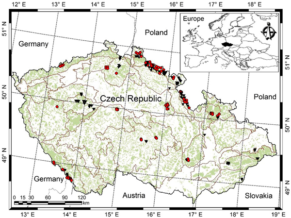
Fig. 1. Location of sample plots [purely Norway spruce or Norway spruce-dominated sample plots (red dots), purely European beech or European beech-dominated sample plots (black triangles), light green shade represents forest cover, and grey lines separating Natural Forest Area].
2.2 Measurements
All measurements were made between April 2007 and August 2015. However, no repeated measurements were involved. Over-bark diameter at breast height (DBH, 1.3 m above ground) was measured with a precision of 1 mm while total height was measured by Laser Vertex with a precision of 0.1 m. Regardless of the species of interest, the position of all living trees with DBH ≥ 4 cm and natural regeneration with DBH < 4 cm and height ≥ 2 m were also recorded. Height to crown base (HCB) for all individuals was measured at the lowest point on the trunk where continuous whorl of at least three living branches was formed, excluding epicormic and adventitious branches. However, this whorl was not considered as a crown base when there were at least three dead whorls above it. Measurements were made for all tree species (1–26 species) on each sample plot. Total height and DBH were measured for all individual trees, regardless of the species, but the crown-width measurements for a few trees were missing on some sample plots. The crown width was measured using the field-map hardware tool (IFER 2009), which is designed for computer-aided dendrometric data collection and data processing. The field crew made projections at four different directions perpendicular to each other on the crown azimuth using this tool. This hardware then automatically computed the circular crown projection area. The coordinates of at least four measured crown edges were connected and smoothed by automatic spline functions in the field-map software. Finally, an area of this figure (crown projection area) was determined and the diameter of the crown calculated as the diameter of a circle, having the same area as the smoothed figure.
3 Data analysis
3.1 Tree and stand characteristics
Stand characteristics such as its development stage, site quality and stand density have substantial influence on the crown of a tree (Hasenauer and Monserud 1996; Fu et al. 2013, 2017; Sharma et al. 2016a), and therefore various stand measures were computed and evaluated for their potential effects on the CDBDR. The site index (dominant height at a reference age), which is commonly used to measure site quality, is included as a predictor in various forest models. However, we could not include the site index in our CDBDR model as this information was not available. Instead, we included the dominant height (HDOM), which was calculated by following the methods suggested by Sharma et al. (2011, 2016a), to describe the combined effects of the stand development stage and site quality. We also evaluated other stand measures, which could have potential effects on the CDBDR, such as number of stems per hectare (N), sum of DBH of all individuals per sample plot (DBHSUM), basal area (BA), basal area of the trees larger in diameter than a subject tree (BAL), arithmetic mean DBH per sample plot (AMD), quadratic mean DBH per sample plot (QMD), and ratio of DBH to QMD. Since the effect of species mixture on tree growth and stand dynamics is substantial (Condés et al. 2013; Sterba et al. 2014; Pretzsch et al. 2015b; Sharma et al. 2016a), this was taken into consideration in our analyses since a major part of our data originated from the mixed stands. We calculated species proportion of the above-mentioned stand measures for the species of interest and evaluated their potential effects on the CDBDR.
3.2 Spatially explicit competition measures
We computed spatially explicit competition measures that describe the competition of neighbors to each subject tree. The missing measurements of crown width of a few trees, including species of interest, prevented us to evaluate distance-weighted ratio of the crown cross-sectional areas or crown volumes of subject trees to their competitors (Biging and Dobbertin 1992; Pretzsch et al. 2002). We chose four commonly used distance-weighted size ratio indices (Eq. 1–4), which are based on the assumption that larger and closer neighbors contribute higher competitive stress to a subject tree.


where CI = competition index, DBH = diameter of a tree at breast height, DIST = distance between subject tree and competitor, n = number of competitors of a subject tree, π = 3.1416, λ = edge expansion factor, s = index for a subject tree, and c = index for a competitor.
We identified all potential competitors within a certain maximum distance around each subject tree using the vertical search angles defined as below (Biging and Dobbertin 1992; Sharma et al. 2016a):
![]()
![]()
where HEIGHTc and HCBs are total height of a competitor c and height to crown base of a subject tree s, respectively, and all other abbreviations and indices are the same as in Eq. 1–4. The alpha (α) is the angle of inclination to the horizontal line, starting from the base of the crown of a subject tree s to the top of a competitor c (Eq. 5), and the theta (θ) is the angle of inclination to the horizontal line, starting from the base of a subject tree s to the top of a competitor c (Eq. 6).
We allowed α and θ to vary from 25° to 70° by 1° increment in Eq. 5 and 6, respectively, which resulted in 360 different CIs. Our analysis involved the examination and comparison of the contributions of all 360 CIs to the CDBDR model using some statistical criteria (to be described later). Hegyi’s index (Eq. 1) computed using the search angle of 50° in Eq. 5 better described competitive situations among the individuals than other alternatives. To reduce potential errors caused by off-plot competitors, we computed linear edge expansion factor as a corrective measure following the methods suggested by Martin et al. (1977) and Goreaud and Pélissier (1999) and adjusted to the competitors.
A statistical summary of the data is presented in Table 1. A monospecific stand includes all individuals other than the species of interest if they had DBH < 4 cm.
| Table 1. Summary statistics of modelling data [CDBDR = ratio of maximum crown diameter to diameter at breast height, in short, crown-to-bole diameter ratio; SD = standard deviation]. | ||
| Variables | Mean ± SD (range) | |
| Norway spruce | European beech | |
| Number of sample plots | 90 (16 monospecific + 74 mixed) | 88 (18 monospecific + 70 mixed) |
| Total number of CDBDR sample trees | 5526 | 5666 |
| Number of CDBDR trees per sample plot | 170 ± 140 (1–450) | 119 ± 81 (1–287) |
| Number of stems per sample plot | 214 ± 105 ( 23–660) | 147 ± 129 (8–677) |
| Number of stems (N ha–1) | 820 ± 472 (86–2581) | 641 ± 474 (34–2685) |
| Stand basal area (BA, m2 ha–1) | 49.7 ± 31 (6.9–81.2) | 55.3 ± 45 (13–81.2) |
| BA proportion of a tree species (BAPOR) | 0.72 ± 0.3 (0.00057–1) | 0.74 ± 0.26 (0.004–1) |
| BA of trees lager than a subject tree (BAL, m2 ha–1) | 34.3 ± 21.4 (0–77.4) | 36 ± 19.2 (0–79.7) |
| Quadratic mean DBH per sample plot (QMD, cm) | 27.4 ± 10.4 (7–60.3) | 34 ± 10.9 (15–66.8) |
| Ratio of DBH to QMD | 1.2 ± 0.5 (0.1–7) | 0.9 ± 0.6 (0.1–5) |
| Arithmetic mean DBH per sample plot (cm) | 24.6 ± 10.8 (6.8–53.9) | 30 ± 11.6 (9–66.3) |
| DBH sum per sample plot (cm) | 4520 ± 1302 (1063–9246) | 3750 ± 1431 (683–9246) |
| Dominant diameter per sample plot (cm) | 46.1 ± 15.2 (9.2–72.8) | 53.6 ± 10.2 (23.4–73) |
| Dominant height per sample plot (HDOM, m) | 25.5 ± 9.3 (6.5–40.4) | 29.2 ± 7.2 (13.3–41.5) |
| Total height (m) | 16.1 ± 10.3 (2–48.7) | 19.6 ± 9.9 (2–48) |
| Ratio of height to diameter (m cm–1) | 0.73 ± 0.22 (0.1–2.1) | 0.74 ± 0.3 (0.1–2.7) |
| Height to crown base (HCB, m) | 5.6 ± 5.5 (0–32.1) | 8.2 ± 6.3 (0–34.1) |
| Crown diameter (m) | 3.6 ± 1.6 (0.7–11.9) | 5.9 ± 2.9 (0.9–19.7) |
| Diameter at breast height (DBH, cm) | 25.4 ± 18.4 (3.1–112) | 29.9 ± 19.4 (3.4–116.1) |
| Crown-to-bole diameter ratio (CDBDR, m cm–1) | 0.2 ± 0.07 (0.04–0.67) | 0.3 ± 0.16 (0.03–0.99) |
No information was recorded by the field crew to differentiate sparse stands from the crowded ones. We could not calculate canopy cover percentage using measurements of crown width (Crookston and Stage 1999) due to missing crown-width measurements of a number of trees. We thus identified sample plots falling either in sparse stands or crowded stands through the subjective judgment of distribution patterns of individuals based on the stem-mapped sample plots. We defined a crowded (or dense) stand sample plot as that which had more than about 70% canopy closure and an open stand sample plot if it had less than this percentage. Our analysis showed 42% of sample plots were in the crowded stands. Graphical displays of CDBDR against DBH by stand openness are shown in Fig. 2.
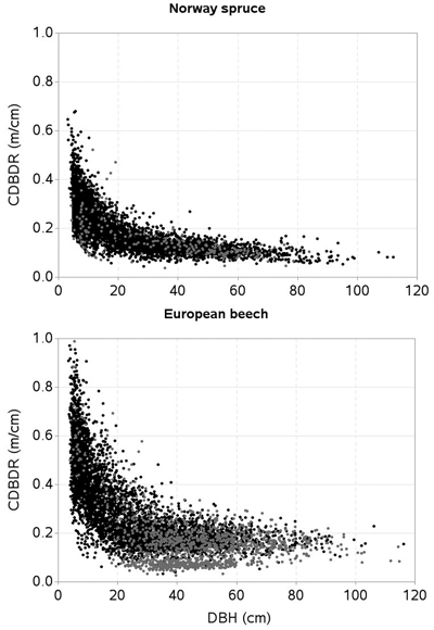
Fig. 2. Crown-to-bole diameter ratio (CDBDR) plotted against diameter at breast height (DBH) of trees [black dots = dense stands; grey dots = sparse stands].
3.3 Modelling approach
The scattered graph shows a strong relationship between CDBDR and DBH (Fig. 2). Considering this figure (i.e. exponential decrease of CDBDR with increasing DBH), we fitted an exponential decay function, hereafter termed as a base model. Among the various formulations evaluated, the following (Eq. 7) provided the smallest sum of squared errors.
![]()
where CDBDRij and DBHij are crown-to-bole diameter ratio and diameter at breast height of a tree j (j = 1,…, m) on sample plot i (i = 1,…, n), respectively, b3 = 0.2, b1 and b2 are parameters, εij is an error term, and m and n are numbers of trees and sample plots, respectively.
Other tree and stand variables and sample plot random effects were also used to expand base model. Among several variables evaluated (Table 1), only significant ones were identified by applying the two-stage variable selection method (Staudhammer and LeMay 2000). This involved fitting the base model by sample plot and examining the scattered-matrix graphs of the values of estimated parameters plotted against each of the potential predictors (Sharma et al. 2016a).The scattered-matrix graph of parameter b1 of the base model (Eq. 7) with respect to HDOM, BAL, BAPOR, and HCB showed significant relationships. Therefore, b1 was then redefined as a function of these variables as shown below:
![]()
where HDOM = dominant height (m); BAL = basal area of trees larger in diameters than a subject tree (m2 ha–1); BAPOR = basal area proportion of a species of interest; HCB = height to crown base (m). The effect of stand openness was also included applying dummy variable modelling, in which b2 of Eq. 7 was redefined as a function of stand openness as shown below:
![]()
We also included sample plot random effects through the mixed-effects modelling. The mixed-effects modelling makes the estimated model subject-specific (sample plot-specific, in our case), resulting in a high prediction accuracy (Pinheiro and Bates 2000). The mixed-effects modelling allows for taking into account the dependency of observations that belong to the same group in the inference following the model fitting (Mehtätalo et al. 2015). The final mixed-effects CDBDR model after inclusion of Eq. 8a and 8b into Eq. 7 is given below:

where z1 = HDOMi, z2 = BALij, z3 = BAPORi, z4 = HCBij, b3 = 0.2, α1,…, α5, φ1, φ2 are parameters; for a sparse stand, openness = 1, 0otherwise. In this equation, HDOMi and BALij are sample plot dominant height (m) and basal area of trees larger in diameters than the jth tree on the ith sample plot (m2 ha–1), respectively; BAPORi and HCBij are basal area proportion based on the species of interest (Norway spruce or European beech) and height to crown base (m) on the ith sample plot, respectively; and, other symbols and acronyms are the same as in Eq. 7. The model (Eq. 9) is henceforth termed as a spatially inexplicit CDBDR model, and the model with BALij replaced by CIij is termed as a spatially explicit CDBDR model. The basic assumptions for the nonlinear mixed effects model (Eq. 9) include the multivariate normal distributions for the random effects vector (ui), residual errors vector (εi) and observations of the response variable vector (CDBDRi). We had no repeated measurements and assumed homoscedasticity in the data.
When b3 was tried to be estimated along with other parameters in Eq. 7 and 9 by optimization, convergence was not achieved. Then, we compared the sum of squared errors (SSE) produced from fitting several alternative values of b3 (0.1 to 2 by 0.1 increment) iteratively, and b3 = 0.2 provided the smallest SSE. The collinearity among the selected predictors was checked using correlation coefficients and only highly significantly contributing predictors were included into the CDBDR model in order to reduce over-parameterization (Montgomery et al. 2001).
3.4 Model estimation and evaluation
Mixed-effects models were estimated with maximum likelihood in SAS macro NLINMIX (SAS Institute Inc. 2013) using the expansion-around-zero method (Littell et al. 2006). However, the best base model was found by considering the fit statistics of the non-linear regression procedure NLIN in SAS (SAS Institute Inc. 2013). The mixed effects model alternatives were evaluated using common statistical criteria such as root mean squared error (RMSE), Akaike information criterion (AIC) (Akaike 1972), and two different coefficient of determinations: marginal coefficient of determination (![]() ) and conditional coefficient of determination (
) and conditional coefficient of determination (![]() ). The (
). The (![]() ) explains fixed effect factors variance and
) explains fixed effect factors variance and ![]() explains variance by both, the fixed and random factors in the mixed effects model (Nakagawa and Schielzeth 2013). The AIC compares the estimated models more logically than any other fit statistics as it is based on the minimizing Kull-back-Lieber distance, and it imposes a penalty for the number of parameters involved in the regression models (Akaike 1972; Burnham and Anderson 2002). Unless otherwise specified, we used 1% level of significance in all analyses and the White test was applied to evaluate variance heteroskedasticity. The effects of each predictor on CDBDR were examined graphically. Even though model validation is important, because it provides credibility and confidence about the model, we were incapable of doing this due to lack of external independent dataset.
explains variance by both, the fixed and random factors in the mixed effects model (Nakagawa and Schielzeth 2013). The AIC compares the estimated models more logically than any other fit statistics as it is based on the minimizing Kull-back-Lieber distance, and it imposes a penalty for the number of parameters involved in the regression models (Akaike 1972; Burnham and Anderson 2002). Unless otherwise specified, we used 1% level of significance in all analyses and the White test was applied to evaluate variance heteroskedasticity. The effects of each predictor on CDBDR were examined graphically. Even though model validation is important, because it provides credibility and confidence about the model, we were incapable of doing this due to lack of external independent dataset.
3.5 Prediction with mixed-effects model
The mixed-effects CDBDR model can be applied for the prediction of CDBDR with or without using the random effects estimated from the measurements of CDBDR of a sub-sample of trees per sample plot. The model without estimated random effects is known as a mean response, while model with estimated random effects is known as a subject-specific model (localized model), and the localizing process is known as calibration (Pinheiro and Bates 2000). A prediction with the former model does not require prior information of a response variable (i.e., CDBDR measured from a sub-sample of trees per sample plot) however, it is required by the latter model. Even though there have been various options reported, generally four or five randomly selected trees per sample plot may be used for unbiased prediction (Calama and Montero 2005; Fu et al. 2013). There is a possibility to localize the mixed-effects CDBDR model using the empirical best linear unbiased prediction method (Pinheiro and Bates 2000; Sirkiä et al. 2015).
4 Results
We developed both the spatially explicit and inexplicit CDBDR model for the Norway spruce and the European beech using DBH and other tree and stand-level measures as predictors through application of the mixed-effects modelling. Among the various potential predictors evaluated (Table 1), dominant height (HDOM), basal area of trees larger in diameter than a subject tree (BAL), basal area proportion of the species of interest (BAPOR), height to crown base (HCB), and Hegyi’s competition index (Eq. 1) appeared to have contributed significantly to the description of the CDBDR variation. Parameter estimates of all predictors including a dummy variable in both spatially explicit and inexplicit models were highly significant (p < 0.0001) and both models described large parts of the CDBDR variation (Table 2). The estimated values and signs of parameters are biologically plausible. For each species, the spatially explicit model better fits the data than its spatially inexplicit counterpart. However, differences between their fit statistics are small.
| Table 2. Parameter estimates, variance components, and fit statistics of the mixed-effects CDBDR model (Eq. 9) [ | ||||
| Model components | Norway spruce | European beech | ||
| Spatially explicit | Spatially inexplicit | Spatially explicit | Spatially inexplicit | |
| Fixed | ||||
| α1 | 2.439952 (0.0962) | 2.010637 (0.0756) | 0.974352 (0.0634) | 1.188444 (0.0750) |
| α2 | 0.079471 (0.00492) | 0.148253 (0.00784) | 0.41734 (0.0155) | 0.368927 (0.014) |
| α3 | –0.02038 (0.00211) | –0.00643 (0.0007) | –0.00932 (0.000965) | –0.01011 (0.000917) |
| α4 | –0.70457 (0.0393) | –0.53672 (0.034) | –0.33188 (0.0573) | –0.46398 (0.0559) |
| α5 | –0.02489 (0.00239) | –0.02571 (0.00248) | –0.08355 (0.00297) | –0.08228 (0.00276) |
| φ1 | 1.431184 (0.0211) | 1.451109 (0.0214) | 1.313027 (0.0199) | 1.27803 (0.0184) |
| φ2 | 0.070045 (0.0114) | 0.056779 (0.0116) | 0.010468 (0.00186) | 0.011452 (0.00153) |
| Variance | ||||
| σ2ui1 | 1.8217 | 2.0167 | 3.1853 | 3.2148 |
| σui1ui2 | –0.4162 | –0.6051 | –0.9902 | –0.7329 |
| σ2ui2 | 0.0926 | 0.1189 | 0.1572 | 0.05182 |
| σ2 | 0.00131 | 0.00142 | 0.00511 | 0.00305 |
| Fit statistics | ||||
| 0.6994 | 0.6849 | 0.7559 | 0.7503 | |
| 0.7286 | 0.7104 | 0.7791 | 0.7657 | |
| RMSE | 0.0349 | 0.0371 | 0.0626 | 0.0653 |
| AIC | –24702 | –24551 | –23931 | –23804 |
The box plots of the residuals show no serious systematic deviation for a majority of the observed data and estimated CDBDR (Fig. 3). However, small deviations in the residuals are seen only for a few large-sized trees. Within-sample plot heteroskedasticity was not significant (p > 0.05: White test), and histograms of the residuals showed a Gaussian distribution pattern (bell-shaped pattern), indicating that skewness was absent in the residuals. Also, no pronounced trend was observed in the residuals plotted by open stands, dense stands, mixed species stands, and monospecific stands, indicating that models adequately fitted to the data acquired from each stand category.
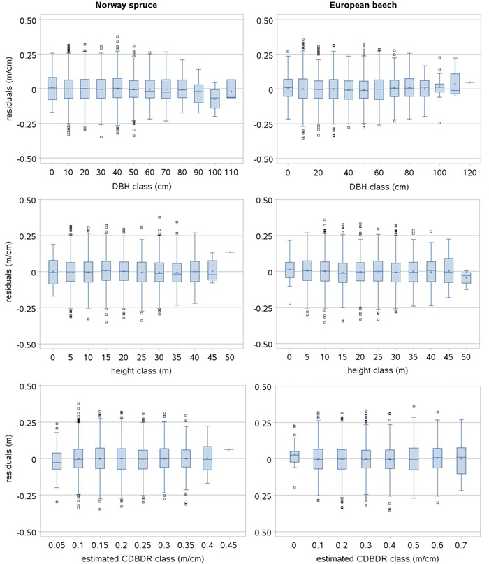
Fig. 3. Box plots of the standardized residuals of the spatially inexplicit crown-to-bole diameter ratio (CDBDR) model (Eq. 9). Length of larger box represents the interquartile range (IQR), length of whisker represents class minimum and maximum values in the IQR, and smaller boxes represent the observations 1.5 times beyond the IQR (outlier observations lying far away from the median) and horizontal lines and plus signs in a larger box represent class median and mean values, respectively.
The effects of the predictors related to tree-size (HCB), stand development stage and site quality (HDOM), competition (BAL, CI), and proportion of the species of interest (BAPOR) on the CDBDR were simulated using both, the spatially inexplicit model (Fig. 4 and 5) and spatially explicit model (Fig. 6). For each species, the effect of HCB emerged as the largest followed by the effect of HDOM, and CDBDR increased with increasing HDOM, but decreased with increasing competition (increased BAL or CI). Also, CDBDR increased with decreasing HCB and increasing species proportion (decreased BAPOR). The effect of each predictor on the CDBDR for open stands only slightly differed from that shown in Figs. 4–6.
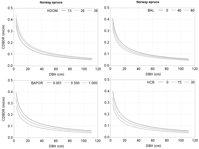
Fig. 4. Effects of dominant height (HDOM), basal area of trees larger in diameters than a subject tree (BAL), basal area proportion of Norway spruce (BAPOR), and height to crown base (HCB) on crown-to bole-diameter ratio (CDBDR). Curves were produced using parameter estimates in Table 2 (spatially inexplicit model for dense stands). Mean values of the data were used as predictors except the variable of interest in each figure, which varied from about minimum to maximum in the data (see Table 1).
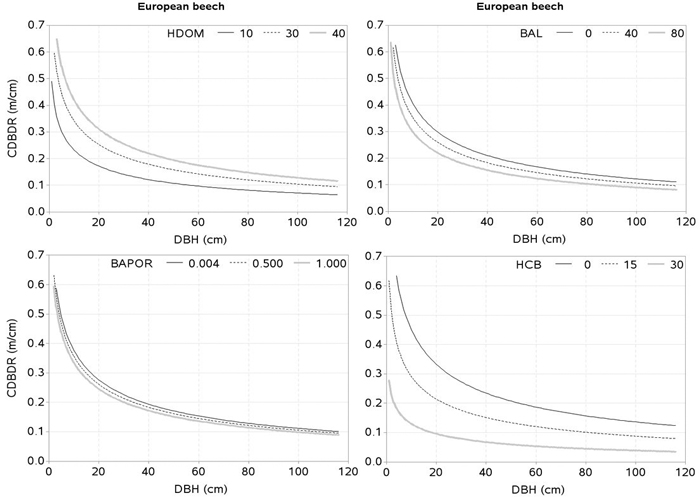
Fig. 5. Effects of dominant height (HDOM), basal area of trees larger in diameters than a subject tree (BAL), basal area proportion of European beech (BAPOR), and height to crown base (HCB) on crown-to bole-diameter ratio (CDBDR). Curves were produced using parameter estimates in Table 2 (spatially inexplicit model for dense stands). Mean values of the data were used as predictors except the variable of interest in each figure, which varied from about minimum to maximum in the data (see Table 1).
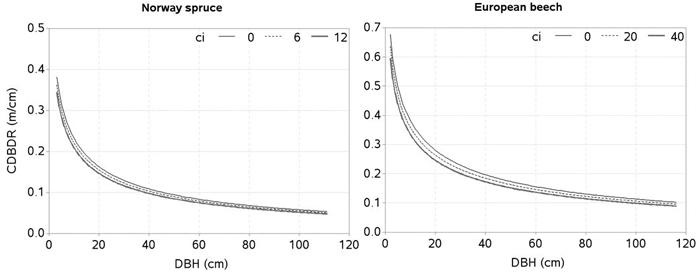
Fig. 6. Effects of spatially explicit competition (CI) on crown-to bole-diameter ratio (CDBDR). Curves were produced using parameter estimates in Table 2 (spatially explicit model for dense stands). Mean values of the data were used as predictors except the variable of interest in each figure, which varied from about minimum to maximum in the data.
5 Discussion
We developed the CDBDR model which is based on a large dataset collected from fully mapped permanent sample plots representing a wide variability of stand density, site quality, and management regime. Knowing that the allometric relationship between crown and DBH would largely vary with tree and stand characteristics (Bragg 2001; Sharma et al. 2016a; Taylor et al. 2016), we developed the CDBDR model using significant tree and stand-wise predictors. Description of a large part of the CDBDR variation without significant trends in the residuals (Table 2, Fig. 3) shows that the base model (Eq. 7) and predictors selected are best suited to our data. Our models also do not exhibit bias for any species-specific stands and forest types, and they behave significantly differently for the trees in sparse and dense stands. This is due to the pronounced effect of stand openness conditions on the CDBDR that was successively modelled with a subjectively defined sparse stand dummy variable. As we defined stand openness by making a subjective judgement on the stem-mapped sample plots, model users also need to make similar judgements when applying the models. Certainly, judgments will differ between the model users. However, we expect that prediction bias will be insignificant even if similar judgements (i.e., a stand with more than 70% canopy cover as a dense stand) are not used when subject-specific predictions are made by applying the localized mixed-effects models. Because, measurements of the crown diameter for sub-sampled trees to be used for prediction of the random effects will be good representative to rest of the trees per sample plot.
As in other studies (Eule 1959, and Freist 1960 in Assmann 1970, p. 109), our data also show that the tree canopy height and their social positions significantly influences the projection ratio or CDBDR (Fig. 7). In this figure, the mean CDBDR for a given crown projection area (CPA) largely varies with three canopy height classes, indicating that social positions of the trees have significant effects on the CDBDR. The extensive data collected from 70 to 170 year-old beech stands (Eule 1959, and Freist 1960 in Assmann 1970) in a given social class, show that the mean CDBDR first increases rapidly but subsequently slowly with increasing the crown projection area. Our data in each canopy height class shows more or less the similar patterns, i.e., increased patterns in general (Fig. 7). A largely reduced CDBDR for any CPA class seen in this figure may be due to few observations. For example, canopy height classes 1, 2 and 3 at the CPAs of 260, 160 and 100 m2 for European beech have 5, 7 and 6 observations, respectively. Assmann (1970) and other studies also show that CDBDR increases on the same screened or shaded areas with decreasing cenotic positions, and CDBDR decreases further with tree ages. However, we could not examine the relationship between CDBDR and age due to tree age data being unavailable. A large fluctuation of CDBDR could occur, for example, in case of a full canopy stand, where tree crowns could not grow laterally, but because of the increased bole diameter, this ratio decreases. After heavy thinning of beech stands, crown width could grow faster than bole diameter, and consequently CDBDR would be larger (Eule 1959, and Freist 1960 in Assmann 1970). Due to the lack of the thinning data, we could not evaluate our models in a similar way.
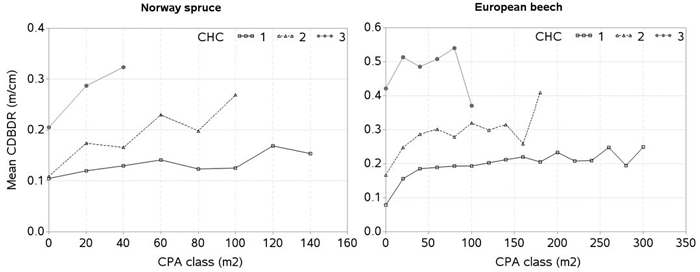
Fig. 7. Mean crown-to-bole diameter ratio (CDBDR) plotted over the crown projection area (CPA) class for each canopy height class (CHC) [mean CDBDR was calculated by CPA class with 20 m2 interval; CHC 1: height > 66% height of the tallest tree, CHC 2: 33% height of the tallest tree < height < 66% height of the tallest tree, and CHC 3: height < 33% height of the tallest tree per sample plot; zero in x-axis stands for CPA class ≤ 10 m2, but > 0 m2].
The effect of HCB on CDBDR is highly significant (Fig. 4 and 5), because it is strongly correlated with crown dimensions (Sharma et al. 2016a). Since crown recession and height growth of trees are two important factors of HCB dynamics, any changes to them result in a significant change on the crown dimensions (Power et al. 2012; Sharma et al. 2016a), and consequently on the CDBDR. When the lower branches die, this results in a crown recession, which leads to a larger HCB and a narrower crown. Crown recession is largely affected by competitive interaction among trees (Valentine et al. 2013), light availability to the lower branches, and physical interactions with neighboring trees. Trees growing in a crowded stand or trees with larger crowns may experience more physical interactions with neighboring trees, resulting in increased crown recession (Power et al. 2012). Crowns of tall trees are also subject to considerable movement due to wind-blow and resulting collisions may lead to substantial abrasion of branches and foliage (Rudnicki et al. 2003). Any change in the HCB may also reflect variability in the epicormic re-sprouting after a canopy loss during a drought period and after snow damages (Taylor et al. 2016).
The crown of a spruce is affected more by air pollution than that of a beech (Vacek et al. 2013), and this may be the reason why the model exhibits a lower HCB effect on the CDBDR for spruce trees compared to beech trees (Fig. 4 and 5). The impact of emissions on spruce trees usually shortens the length of the crown; the crowns are dried mainly from the bottom where they are the widest, therefore increasing the crown height; and significantly less drying of the crown from the top or around the circumference (Vacek et al. 2015a) may result in a considerably reduced crown width. However, the crown of a beech tree within in a stand suffers from the drying up or the dehydration of individual branches, which has little effect on the crown width (Vacek 1988). Other factors and management interventions also affect HCB, which in turn, substantially affects tree growth and stand dynamics. The HCB is commonly used as a predictor in various forest models including crown models (Ritson and Sochacki 2003; Fu et al. 2013, 2017; Sharma et al. 2016a).
Few crown-modelling studies (e.g., Fu et al. 2013, 2017; Sharma et al. 2016a) have assumed HDOM as a measure of site quality, which is not an appropriate assumption; because the same HDOM can be found in younger stands with better site quality and older stands with poorer site quality. Therefore, HDOM better reflects the stand development stage rather than site quality. However, we considered HDOM as a measure that could describe the combined effects of both, the stand development stage and site quality. Due to lack of site index data, we used HDOM for this purpose. The HDOM showed a significant effect on the CDBDR (Fig. 4 and 5). Growth modelling studies often show significant relationships between HDOM, growth of the trees and stand dynamics. Inclusion of HDOM in the CDBDR model may be justifiable, because it reflects stand growth and yield development. It is also easier to measure than site index. For a given competitive situation among the trees in a stand, CDBDR increases with increasing HDOM. This may be plausible for better sites where availability of more resources helps accelerate growth and crown expansion of the trees.
Tree crowns are largely affected by competitive interactions among the trees (Thorpe et al. 2010; Sharma et al. 2016a). We found, much like other studies (Hasenauer and Monserud 1996; Contreras et al. 2011), the basal area of trees larger in diameter than a subject tree (BAL) better describes the competition responses than any other inexplicit measures. For a given HDOM, our models exhibit decreased CDBDR with increasing BAL (Fig . 4 and 5) and Hegyi’s competition index (Fig. 6). This is due to increased crowding of individuals in a stand that results in taller height, narrower crown, and thinner stem, but larger HCB (Bragg 2001; Sharma et al. 2016a). Suppressed trees attempting to reach higher canopy positions would have less growth in diameter than height for a given unit of crown size as compared to trees already grown to the top canopy position (Wonn and O’Hara 2001; Sharma et al. 2016b), which may result in a larger CDBDR. Suppressed trees are able to allocate more resources to height growth and crown expansion relative to diameter growth (Wonn and O’Hara 2001). Trees with very large CDBDR may be possible in extremely sparse stands, but our data does not indicate this (Fig. 2) as sample plots were not located in extremely sparse stands (i.e., no sample plot had less than 30% canopy closure).
Competition indices computed using tree positioning may better describe competitive interactions among the trees than those computed without tree positioning (Biging and Dobbertin 1992; Pretzsch 2009; Sharma et al. 2016a). This explains why our spatially explicit model better fits the data (Table 2). However, some other studies, (e.g. Lorimer 1983; Martin and Ek 1984) found spatially inexplicit competition indices (e.g. stand basal area) to be superior to spatial competition indices when modelling tree growth. Competition is a continuous, complex, and dynamic process, which is indirectly assessed using various competition indices. Most of these indices focus only on the aboveground competition as the primary determinant of growth, when belowground competition is likely to be equally or more important (Coomes and Grubb 2000; Weiskittel et al. 2011). Thus, a single index of competition cannot holistically represent all components of competition. Furthermore, competition indices describe growth and other tree characteristics differently as competition varies with stand density, species composition, tree size, site quality, and stand structures (Pretzsch 2009; Contreras et al. 2011; Sharma et al. 2016a, 2016b). Inclusion of species-specific competition effects (Pretzsch et al. 2002; Thorpe et al. 2010), and other characteristics within the competition indices, are rarely practiced because of computational complexity. This study only used height and DBH in the competition indices (Eq. 1–6) in order to make the CDBDR model simpler. Application of spatially explicit models need information from the individual tree positions, which may not be obtained from routine forest inventories as they are costly. However, it could become more accessible and more affordable when spatial data from airborne laser scanning (Hyyppa et al. 2012), or data generated based on the empirical spatial distribution patterns (Pretzsch 1997), becomes available.
The effect of species mixture (BAPOR) on the CDBDR model is highly significant (p < 0.0001). For a given competitive situation and HDOM, CDBDR decreases with decreasing proportion of the species of interest (Fig. 4 and 5). Species mixture creates a neighborhood situation, where wider crown width is possible (Bayer et al. 2013). A tree crown is formed under the influence of local environment and availability of growth resources, which is determined by intra- or inter-specific interactions of the trees (Bayer et al. 2013; Pretzsch et al. 2015b; Sharma et al. 2016a). The structural difference of crowns in monospecific and mixed stands is significant, which can be due to differences in canopy space-filling and resource use efficiency (Pretzsch 2014; Pretzsch et al. 2015b). Space-filling within a crown, such as angle, length, number, and ramification of branches in the mixed stands, may differ from those in monospecific stands, which may result in significant changes in resource supply and resource use efficiency (Pretzsch 2009; Bayer et al. 2013; Pretzsch 2014; Pretzsch et al. 2015b). Therefore, a better understanding of the effects of species mixture on tree growth and stand dynamics is important for decision-making in forestry.
The CDBDR provides the information of crown dynamics in various development stages of a tree, and therefore it has silvicultural importance. Even though various applications of CDBDR are available (Dawkins 1963; Seebach 1845; Eule 1959, and Freist 1960 in Assmann 1970; Ayhan 1974; Hemery et al. 2005), they all have lacked in-depth analyses of the factors that can affect the CDBDR. The CDBDR may be used to assess the stability of the individual trees and stands of the species of interest. The CDBDR model can be used as input to tree growth simulators to be developed in the future. The CDBDR model may be a part of the future forest risk model, which integrates all potential risk factors including climate, and may be used to assess overall risk for stand stability. A forest risk model may be of great importance in the Czech Republic, where static stability of spruce stands are low. For example, 17% of salvage cutting was caused by abiotic factors such as wind, snow and icing in 2014, but approximately 73% of the total damage was mainly caused by wind (MA 2015). Considerable incidents of stand damages can be expected in the future due to less static stability of conifer stands and increased fluctuations of weather.
6 Conclusion
The spatially explicit CDBDR model showed slightly more attractive fit statistics than those of its spatially inexplicit counterpart, though differences were small. Model users, therefore, may prefer an application of the spatially inexplicit model as it does not require the Hegyi’s competition index, which requires tree mapping and is computationally more complex than basal area of trees larger in diameter than a subject tree. When a detailed description of the stand structure and a high prediction accuracy is required, application of the spatially explicit model should be the preferred choice. The CDBDR can be useful in describing stand density and growing stock of the stands. The CDBDR model may have various management implications such as determination of spacing, stand basal area, stocking, and planning of appropriate species mixture. Recalibration of the CDBDR model using site index and longer time-series data will be more useful as these data better describe site quality, stand management history and changing patterns of the crown dimensions over the years.
Acknowledgements
This study was supported by Ministry of Agriculture of the Czech Republic (No. QJ1520037) and Faculty of Forestry and Wood Sciences (FLD) in the Czech University of Life Sciences (CULS) in Prague (Excellent Output Project-2016, IGA projects: A03/17 and B03/17). This work was also supported by EXTEMIT- K project (No. CZ.02.1.01/0.0/0.0/15_003/0000433 financed by OP RDE) in FLD, CULS. We are grateful to three reviewers and editor for their constructive comments and valuable suggestions that helped improve the manuscript.
References
Akaike H. (1972). A new look at statistical model identification. IEEE Trans Autom Control AC19: 716–723.
Alemdag I.S. (1978). Evaluation of some competition indices for the prediction of diameter growth in planted white spruce. Canadian Forestry Service, Forest Management Institute, Ottawa, Ontario. Information Report FMR-X-108. 39 p.
Assmann E. (1970). The principles of forest yield studies. Pergamon press, Oxford. 506 p.
Avery T.E., Burkhart H.E. (2002). Forest measurements (5th ed.). McGraw-Hill Inc., NY.
Ayhan H.O. (1974). Crown diameter: dbh relations in Scots pine. Arbor 5: 15–25.
Bayer D., Seifert S., Pretzsch H. (2013). Structural crown properties of Norway spruce (Picea abies [L.] Karst.) and European beech (Fagus sylvatica [L.]) in mixed versus pure stands revealed by terrestrial laser scanning. Trees 27(4): 1035–1047. https://doi.org/10.1007/s00468-013-0854-4.
Biging G.S., Dobbertin M. (1992). Comparison of distance-dependent competition measures for height and basal area growth of individual conifer trees. Forest Science 38: 695–720.
Bragg D.C. (2001). A local basal area adjustment for crown width prediction. Northern Journal of Applied Forestry 18: 22–28.
Buckley T.N., Cescatti A., Farquhar G.D. (2013). What does optimization theory actually predict about crown profiles of photosynthetic capacity when models incorporate greater realism? Plant, Cell & Environment 36: 1547–1563. https://doi.org/10.1111/pce.12091.
Burnham K.P., Anderson D.R. (2002). Model selection and inference: a practical information-theoretic approach. Springer-Verlag, New York.
Calama R., Montero G. (2005). Multilevel linear mixed model for tree diameter increment in stone pine (Pinus pinea): a calibrating approach. Silva Fennica 39(1): 37–54. https://doi.org/10.14214/sf.394.
Carvalho J.P., Parresol B.R. (2003). Additivity in tree biomass components of Pyrenean oak (Quercus pyrenaica Willd.). Forest Ecology and Management 179(1–3): 269–276. https://doi.org/10.1016/S0378-1127(02)00549-2.
Condés S., Del Rio M., Sterba H. (2013). Mixing effect on volume growth of Fagus sylvatica and Pinus sylvestris is modulated by stand density. Forest Ecology and Management 292: 86–95. https://doi.org/10.1016/j.foreco.2012.12.013.
Contreras M.A., Affleck D., Chung W. (2011). Evaluating tree competition indices as predictors of basal area increment in western Montana forests. Forest Ecology and Management 262(11): 1939–1949. https://doi.org/10.1016/j.foreco.2011.08.031.
Coomes D.A., Grubb P.J. (2000). Impacts of root competition in forests and woodlands: a theoretical framework and review of experiments. Ecological Monographs 70(2): 171–207. https://doi.org/10.1890/0012-9615(2000)070[0171:IORCIF]2.0.CO;2.
Crookston N.L., Stage A.R. (1999). Percent canopy cover and stand structure statistics from the Forest Vegetation Simulator. U.S. Forest Service, General Technical Report, RMRS-GTR-24. 11 p. https://doi.org/10.2737/RMRS-GTR-24.
Dawkins H.C. (1963). Crown diameters: their relation to bole diameter in tropical forest trees. Commonwealth Forestry Review 42: 318–333.
Deleuze C., Hervé J.-C., Colin F., Ribeyrolles L. (1996). Modelling crown shape of Picea abies: spacing effects. Canadian Journal of Forest Research 26(11): 1957–1966. https://doi.org/10.1139/x26-221.
Foli E.G., Alder D., Miller H.G., Swaine M.D. (2003). Modelling growing space requirements for some tropical forest tree species. Forest Ecology and Management 173(1-3): 79–88. https://doi.org/10.1016/S0378-1127(01)00815-5.
Fu L., Sun H., Sharma R.P., Lei Y., Zhang H., Tang S. (2013). Nonlinear mixed-effects crown width models for individual trees of Chinese fir (Cunninghamia lanceolata) in south-central China. Forest Ecology and Management 302: 210–220. https://doi.org/10.1016/j.foreco.2013.03.036.
Fu L., Sharma R.P., Hao K., Tang S. (2017). A generalized interregional nonlinear mixed-effects crown width model for Prince Rupprecht larch in northern China. Forest Ecology and Management 389: 364–373. https://doi.org/10.1016/j.foreco.2016.12.034.
Goreaud F., Pélissier R. (1999). On explicit formulae of edge effect correction for Ripley’s K-function. Journal of Vegetation Science 10: 433–438. https://doi.org/10.2307/3237072.
Grote R. (2003). Estimation of crown radii and crown projection area from stem size and tree position. Annals of Forest Science 60(5): 393–402. https://doi.org/10.1051/forest:2003031.
Hasenauer H., Monserud R.A. (1996). A crown ratio model for Austrian forests. Forest Ecology and Management 84(1–3): 49–60. https://doi.org/10.1016/0378-1127(96)03768-1.
Hasenauer H., Monserud R.A. (1997). Biased predictions for tree height increment models developed from smoothed ‘data’. Ecological Modelling 98(1): 13–22. https://doi.org/10.1016/S0304-3800(96)01933-3.
Hegyi F. (1974). A simulation model for managing jack-pine stands. In: Fries J. (ed.). Growth models for tree and stand simulation. Royal College of Forestry, Stockholm, Sweden. Research Note 30. p. 74–90.
Hemery G.E., Savill P.S., Pryor S.N. (2005). Applications of the crown diameter-stem diameter relationship for different species of broadleaved trees. Forest Ecology and Management 215(1–3): 285–294. https://doi.org/10.1016/j.foreco.2005.05.016.
Hyyppä J., Holopainen M., Olsson H. (2012). Laser scanning in forests. Remote Sensing 4(10): 2919–2922. https://doi.org/10.3390/rs4102919.
IFER (Institute of Forest Ecosystem and Research) (2009). Tool designed for computer aided field data, Technology Field-Map. IFER: Monitoring and Mapping Solutions, Ltd. Jílové u Prahy. 30 p.
Kuprevicius A., Auty D., Achim A., Caspersen J.P. (2014). Quantifying the influence of live crown ratio on the mechanical properties of clear wood. Forestry 86(3): 449–458. https://doi.org/10.1093/forestry/cpt006.
Lappi J. (1991). Calibration of height and volume equations with random parameters. Forest Science 37(3): 781–801.
Lappi J., Bailey R.L. (1988). A height prediction model with random stand and tree parameters: an alternative to traditional site index methods. Forest Science 34(4): 907–927.
Lindstrom J.M., Bates D.M. (1990). Non-linear mixed-effectss models for repeated measures data. Biometrics 46(3): 673–687. https://doi.org/10.2307/2532087.
Littell R.C., Milliken G.A., Stroup W.W., Wolfinger R.D., Schabenberger O. (2006). SAS for mixed models, 2nd ed. SAS Institute, Cary, NC. 814 p.
Long J.N., Vacchiano G. (2014). A comprehensive framework of forest stand property–density relationships: perspectives for plant population ecology and forest management. Annals of Forest Science 71(3): 325–335. https://doi.org/10.1007/s13595-013-0351-3.
Lorimer C.G. (1983). Test of age-independent competition indices for individual trees in natural hardwood stands. Forest Ecology and Management 6(4): 343–360. https://doi.org/10.1016/0378-1127(83)90042-7.
MA (Ministry of Agriculture) (2015). Report on the state of forests and forest management in the Czech Republic in 2014. Ministry of agriculture, Prague. 108 p.
Martin G.L., Ek A.R. (1984). A comparison of competition measures and growth models for predicting plantation red pine diameter and height growth. Forest Science 30: 731–743.
Martin G.L., Ek A.R., Monserud R.A. (1977). Control of plot edge bias in forest stand growth simulation models. Canadian Journal of Forest Research 7(1): 100–105. https://doi.org/10.1139/x77-014.
Mehtätalo L., de-Miguel S., Gregoire T.G. (2015). Modeling height-diameter curves for prediction. Canadian Journal of Forest Research 45(7): 826–837. https://doi.org/10.1139/cjfr-2015-0054.
Meng S.X., Huang S.M., Yang Y.Q., Trincado G., VanderSchaaf C.L. (2009). Evaluation of population-averaged and subject-specific approaches for modeling the dominant or codominant height of lodge-pole pine trees. Canadian Journal of Forest Research 39(6): 1148–1158. https://doi.org/10.1139/x09-039.
Monserud R.A., Sterba H. (1996). A basal area increment model for individual trees growing in even- and uneven-aged forest stands in Austria. Forest Ecology and Management 80(1–3): 57–80. https://doi.org/10.1016/0378-1127(95)03638-5.
Monserud R.A., Sterba H. (1999). Modeling individual tree mortality for Austrian forest species. Forest Ecology and Management 113(2–3): 109–123. https://doi.org/10.1016/S0378-1127(98)00419-8.
Montgomery D.C., Peck E.A., Vining G.G. (2001). Introduction to linear regression analysis. New York, Wiley. 641 p.
Nakagawa S., Schielzeth H. (2013). A general and simple method for obtaining R2 from generalized linear mixed-effects models. Methods in Ecology and Evolution 4(2): 133–142. https://doi.org/ 10.1111/j.2041-210x.2012.00261.x.
Pinheiro J.C., Bates D.M. (2000). Mixed-effects models in S and S-PLUS. Springer, New York.
Porte A., Bartelink H.H. (2002). Modelling mixed forest growth: a review of models for forest management. Ecological Modelling 150(1–2): 141–188. https://doi.org/10.1016/s0304-3800(01)00476-8.
Power H., LeMay V., Berninger F., Sattler D., Kneeshaw D. (2012). Differences in crown characteristics between black (Picea mariana) and white spruce (Picea glauca). Canadian Journal of Forest Research 42(9): 1733–1743. https://doi.org/10.1139/x2012-106.
Pretzsch H. (1997). Analysis and modeling of spatial stand structures. Methodological considerations based on mixed beech-larch stands in Lower Saxony. Forest Ecology and Management 97(3): 237–253. https://doi.org/10.1016/s0378-1127(97)00069-8.
Pretzsch H. (2009). Forest dynamics, growth and yield: from measurement to model. Springer-Verlag, Berlin. 664 p.
Pretzsch H. (2014). Canopy space filling and tree crown morphology in mixed-species stands compared with monocultures. Forest Ecology and Management 327: 251–264. https://doi.org/10.1016/j.foreco.2014.04.027.
Pretzsch H., Biber P., Dursky J. (2002). The single tree-based stand simulator SILVA: construction, application and evaluation. Forest Ecology and Management 162(1): 3–21. https://doi.org/10.1016/S0378-1127(02)00047-6.
Pretzsch H., Biber P., Uhl E., Dahlhausen J., Rötzer T., Caldentey J., Koike T., van Con T., Chavanne A., Seifert T., Toit B., Farnden C., Pauleit S. (2015a). Crown size and growing space requirement of common tree species in urban centers, parks, and forests. Urban Forestry and Urban Greening 14(3): 466–479. https://doi.org/10.1016/j.ufug.2015.04.006.
Pretzsch H., Forrester D.I., Rötzer T. (2015b). Representation of species mixing in forest growth models. A review and perspective. Ecological Modelling 313: 276–292. https://doi.org/10.1016/j.ecolmodel.2015.06.044.
Pretzsch H., Schutze G. (2005). Crown allometry and growing space efficiency of Norway spruce (Picea abies L. Karst.) and European beech (Fagus sylvatica L.) in pure and mixed stands. Plant Biology 7: 628–639. https://doi.org/10.1055/s-2005-865965.
Pukkala T. (1989). Methods to describe the competition process in a tree stand. Scandinavian Journal of Forest Research 4(1–4): 187–200. https://doi.org/10.1080/02827588909382557.
Ritson P., Sochacki S. (2003). Measurement and prediction of biomass and carbon content of Pinus pinaster trees in farm forestry plantations, south-western Australia. Forest Ecology and Management 175(1–3): 103–117. https://doi.org/10.1016/S0378-1127(02)00121-4.
Rudnicki M., Lieffers V.J., Silins U. (2003). Stand structure governs the crown collisions of lodgepole pine. Canadian Journal of Forest Research 33(7): 1238–1244. https://doi.org/10.1139/x03-055.
SAS Institute Inc. (2013). Base SAS 9.4 Procedure guide: statistical procedures. 2nd ed. SAS Institute Inc., Carry. 556 p.
Schmidt M., Hanewinkel M., Kändler G., Kublin E., Kohnle U. (2010). An inventory-based approach for modeling single-tree storm damage- an experiences with the winter storm of 1999 in southwestern Germany. Canadian Journal of Forest Research 40(8): 1636–1652. https://doi.org/10.1139/X10-099.
Sharma R.P., Breidenbach J. (2015). Modeling height-diameter relationships for Norway spruce, Scots pine, and downy birch using Norwegian national forest inventory data. Forest Science and Technology 11(1): 44–53. https://doi.org/10.1080/21580103.2014.957354.
Sharma R.P., Brunner A., Eid T., Øyen B.-H. (2011). Modelling dominant height growth from national forest inventory individual tree data with short time series and large age errors. Forest Ecology and Management 262(12): 2162–2175. https://doi.org/10.1016/j.foreco.2011.07.037.
Sharma R.P., Vacek Z., Vacek S. (2016a). Individual tree crown width models for Norway spruce and European beech in Czech Republic. Forest Ecology and Management 366: 208–220. https://doi.org/10.1016/j.foreco.2016.01.040.
Sharma R.P., Vacek Z., Vacek S. (2016b). Modeling individual tree height to diameter ratio for Norway spruce and European beech in Czech Republic. Trees 30(6): 1969–1982. https://doi.org/10.1007/s00468-016-1425-2.
Sirkiä S., Heinonen J., Miina J., Eerikäinen K. (2015). Subject-specific prediction using a nonlinear mixed model: consequences of different approaches. Forest Science 61(2): 205–212. https://doi.org/10.5849/forsci.13-142.
Šmelko Š.S., Merganič J. (2008). Some methodological aspects of the national forest inventory and monitoring in Slovakia. Journal of Forest Science 54: 476–483.
Soares P., Tomé M. (2001). A tree crown ratio prediction equation for eucalypt plantations. Annals of Forest Science 58(2): 193–202. https://doi.org/10.1051/forest:2001118.
Staudhammer C., LeMay V. (2000). Height prediction equations using diameter and stand density measures. The Forestry Chronicle 76(2): 303–309. https://doi.org/10.5558/tfc76303-2.
Sterba H., Rio M., Brunner A., Condes S. (2014). Effect of species proportion definition on the evaluation of growth in pure vs. mixed stands. Forest Systems 23(3): 547–559. https://doi.org/10.5424/fs/2014233-06051.
Tahvanainen T., Forss E. (2008). Individual tree models for the crown biomass distribution of Scots pine, Norway spruce and birch in Finland. Forest Ecology and Management 255(3–4): 455–467. https://doi.org/10.1016/j.foreco.2007.09.035.
Taylor J.E., Ellis M.V., Rayner L., Ross K.A. (2016). Variability in allometric relationships for temperate woodland Eucalyptus trees. Forest Ecology and Management 360: 122–132. https://doi.org/10.1016/j.foreco.2015.10.031.
Temesgen H., LeMay V., Mitchell S.J. (2005). Tree crown ratio models for multi-species and multi-layered stands of southeastern British Columbia. The Forestry Chronicle 81(1): 133–141. https://doi.org/10.5558/tfc81133-1.
Thorpe H.C., Astrup R., Trowbridge A., Coates K.D. (2010). Competition and tree crowns: a neighborhood analysis of three boreal tree species. Forest Ecology and Management 259(8): 1586–1596. https://doi.org/10.1016/j.foreco.2010.01.035.
Vacek S. (1988). Dynamics of the defoliation of beech forest stands under the influence of air pollution. In: 3. IUFRO Buchensymposium, Zvolen, 3.6–6.6. 1988. Zvolen, VŠLD. p. 377–388.
Vacek S., Bílek L., Schwarz O., Hejcmanová P., Mikeska M. (2013). Effect of air pollution on the health status of Spruce stands. Mountain Research and Development 33(1): 40–50. https://doi.org/10.1659/mrd-journal-d-12-00028.1.
Vacek S., Hůnová I., Vacek Z., Hejcmanová P., Podrázský V., Král J., Putalová T., Moser W.K. (2015a). Effects of air pollution and climatic factors on Norway spruce forests in the Orlické hory Mts. (Czech Republic), 1979–2014. European Journal of Forest Research 134(6): 1127–1142. https://doi.org/10.1007/s10342-015-0915-x.
Vacek Z., Vacek S., Bílek L., Remeš J., Štefančík I. (2015b). Changes in horizontal structure of natural beech forests on an altitudinal gradient in the Sudetes. Dendrobiology 73: 33–45. https://doi.org/10.12657/denbio.073.004.
Valentine H.T., Amateis R.L., Gove J.H., Mäkelä A. (2013). Crown-rise and crown-length dynamics: application to loblolly pine. Forestry 86(3): 371–375. https://doi.org/10.1093/forestry/cpt007.
Weiskittel A.R., Hann D.W., Kershaw J.A. Jr, Vanclay J.K. (2011). Forest growth and yield modeling. Wiley, New York. 424 p. https://doi.org/10.1002/9781119998518.
Wonn H.T., O’Hara K.L. (2001). Height: diameter ratios and stability relationships for four northern rocky mountain tree species. Western Journal of Applied Forestry 16: 87–94.
Total of 80 references.
