
Riku Tarvainen  ,
Kirsi Riekki,
Heikki Ovaskainen,
Kalle Kärhä,
Jukka Malinen
,
Kirsi Riekki,
Heikki Ovaskainen,
Kalle Kärhä,
Jukka Malinen
Strip-road tree identification and stand structure estimation using harvester data
Tarvainen R., Riekki K., Ovaskainen H., Kärhä K., Malinen J. (2026). Strip-road tree identification and stand structure estimation using harvester data. Silva Fennica vol. 60 no. 3 article id 26021. https://doi.org/10.14214/sf.26021
Highlights
- Three methods for identifying strip-road trees from hpr data with accurate positioning were compared
- Inner-stand spatial arrangement of trees and strip-road sampling sensitivity were quantified using theoretical strip-road layouts
- Harvester-based strip-road sampling offers a practical and cost-efficient alternative for forest inventory, but estimates based solely on realised strip-road locations may be biased in certain stand conditions.
Abstract
Harvester data are a potentially valuable source of detailed information on forest inventory in first-thinning stands. In first-thinning operations performed using modern cut-to-length harvesters, all the trees within the strip roads are removed. The resulting systematic strip road network covers approximately 15–20% of the stand area. We investigated how strip-road trees can be identified from harvested production data to quantify within-stand variation and evaluate how strip-road sample placement affects the representativeness of the sample. Three different strip-road tree identification methods were evaluated: (1) a boom-angle and -length method; (2) a buffer method using reconstructed strip-road centrelines in a global coordinate system; and (3) a boom-angle method. The accuracy of the resulting diameter distributions, stem counts and basal-area estimates was assessed using Reynold’s error index and root mean square error metrics against detailed field reference data. In addition, theoretical offset strip roads were established and systematically shifted across each measurement area to quantify within-stand variation and sampling sensitivity. The most accurate stem count estimates were obtained using the boom-angle and -length method and the buffer method, whereas the boom-angle sector method performed poorly. Offset strip-road tree samples revealed substantial variation in stem count and basal area in some stands, indicating that strip-road alignment and spatial heterogeneity can significantly influence the representativeness of the sample. Our findings show that, in general, harvester-based strip-road sampling is a feasible and cost-efficient approach for estimating stand-level forest variables in first thinnings if tree identification methods and spatial biases are carefully considered.
Keywords
simulation;
sampling;
harvester data;
accurate positioning
-
Tarvainen,
Metsäteho Oy, Vernissakatu 1, FI-01300 Vantaa, Finland
 https://orcid.org/0009-0001-2336-3125
E-mail
riku.tarvainen@metsateho.fi
https://orcid.org/0009-0001-2336-3125
E-mail
riku.tarvainen@metsateho.fi
-
Riekki,
Metsäteho Oy, Vernissakatu 1, FI-01300 Vantaa, Finland
https://orcid.org/0009-0007-8366-3297
E-mail
kirsi.riekki@metsateho.fi
-
Ovaskainen,
Metsäteho Oy, Vernissakatu 1, FI-01300 Vantaa, Finland
https://orcid.org/0000-0001-5063-6662
E-mail
heikki.ovaskainen1@gmail.com
- Kärhä, University of Eastern Finland, School of Forest Sciences, Faculty of Science, Forestry and Technology, P.O. Box 111, FI-80101 Joensuu, Finland E-mail kalle.karha@uef.fi
-
Malinen,
Metsäteho Oy, Vernissakatu 1, FI-01300 Vantaa, Finland
https://orcid.org/0000-0002-5023-1056
E-mail
jukka.malinen@metsateho.fi
Received 27 March 2026 Accepted 8 August 2026 Published 20 August 2026
Views 6391
Available at https://doi.org/10.14214/sf.26021 | Download PDF

Supplementary Files
1 Introduction
In even-aged forest management, first thinning is a vital operation, the aim of which is usually to remove the lower-quality trees, open growth space for the most valuable trees and leave an even spatial distribution between the trees. For example, in Finland, first thinning is recommended in Scots pine (Pinus sylvestris L.), Norway spruce (Picea abies (L.) H. Karst.) and birch (Betula pendula Roth) forests when the dominant tree heights reach 13–16 m, the recommended density being 700–1300 trees ha–1 after thinning (Tapio Oy 2025). In Finland, around 150 000 ha of forest are subjected to first thinning annually (Natural Resources Institute Finland Statistics Database 2026). The stem count and basal area are either observed manually or estimated through a range of methods.
Over the last few decades, remote-sensing technologies have developed rapidly. Aerial photogrammetry and satellite imagery provide high spatial and temporal resolution to allow the mapping of large and remote areas. Unmanned aerial vehicles carrying LiDAR or RGB sensors, enable the collection of point cloud data and images for photogrammetry across a range of scales. However, these approaches also have limitations, including low resolution, systematic bias and measurement errors, which reduce their reliability for use in small-scale forest inventories (Sagar et al. 2026; Kangas et al. 2018). On the other hand, open forest inventory data provide average stand-level variables, but diameter distributions are not included. Furthermore, the accuracy of forest variables is generally lower in young and mixed stands, and especially in first thinnings (Finnish Forest Centre 2023).
Modern harvesters are equipped with multiple sensors that enable detailed data acquisition from felled trees (Kärhä et al. 2025). Information, such as stem diameter and length of the commercial part of the stem, are recorded in the harvested production (hpr) file following the StanForD 2010 standard (Skogforsk 2025). In addition, the harvesters are equipped with Global Navigation Satellite System (GNSS) positioning equipment, often with real-time kinematic (RTK) correction, which requires multiple known reference points to correct errors in the satellite signals (Kaartinen et al. 2015). However, this allows for accurate positioning of both the harvester machine and the boom tip. The positioning accuracy of the boom tip varies, ranging from a couple of metres up to 9 metres when using recreational-level GNSS receivers (Kaartinen et al. 2015), but improves substantially with RTK correction, reaching approximately 0.5 m under forest canopy (Hannrup and Möller 2022; Cho et al. 2024; Ylä-Pöntinen et al. 2025).
The position of the harvester boom tip is measured by sensors on the boom joints relative to the harvester cabin. Furthermore, the position of the harvester head is derived from the boom tip and can generally be determined with good accuracy. The boom typically extends to 10–11 m and, ideally, the harvester-head position corresponds to the location of the felled tree. In practice, however, determining this location precisely requires accounting for the geometry of the boom and harvester head, as well as the radius of the felled tree (Ylä-Pöntinen et al. 2025).
In the quality reporting of first thinnings, RTK harvester data can be used to provide valuable insights into forests (Lindroos et al. 2015). Studies have shown that estimating forest variables after thinning is possible when strip-road trees are identified (Bhuiyan et al. 2016; Tarvainen et al. 2025). All trees along the strip roads must be removed to allow machine movement and operation, and this process provides a reasonably large sample of 15–20% of the trees and the stand structure in the harvested area. In addition to the large sample size, strip roads present a systematic layout that can reduce variance compared to the random sampling with small sample plots (Brus 2019), resulting in more accurate estimates under certain spatial conditions. However, although this sample can provide substantial spatial coverage of the stand, it does not constitute a statistically representative sample in the design-based sense (Cochran 1977).
To estimate a stand-wise pre-harvest diameter distribution, stem count and basal area, the strip-road trees identified from the hpr data are scaled to hectare-wise density using the strip-road area, calculated from its width and length. This scaled density serves as the pre-operation estimate for the whole stand. The remaining stem count after thinning is then estimated by subtracting the total hectare-wise hpr data from that pre-operation estimate (Tarvainen et al. 2025). In terms of the accuracy of the stem count and basal area estimates, it is crucial to identify the removed trees correctly using the harvester head position data and the strip-road area. In Skogforsk’s hprGallring method (Bhuyian 2016), the harvester data was used together with other, pre-known, forest attributes, whereas Tarvainen et al. (2025) used only the harvester data. The main difference between these two methods is the identification of the strip-road trees. In Skogforsk’s method, the strip-road trees were identified based only on the boom angle (Bhuyian 2016; Möller 2024), whereas Tarvainen et al. (2025) used both the boom angle and its length to calculate the distance of each felled tree from the strip-road centreline, and thus identify all the strip-road trees. A recent SLU master’s thesis evaluated hprGallring against manual circular-plot inventory in ten first-thinned stands in northern Sweden, reporting comparable estimates of stem count, basal area and volume at the population level, although with considerable variation between individual stands. Stem count differed by –32.0% to 32.2% (20.1% standard deviation of the differences), basal area by –15.3% to 19.6% (10.6%), and volume by –17.4% to 27.7% (13.3%) compared with the field reference (Källmark 2025).
The alignment of the strip roads may also affect the estimation of forest variables when using the known strip-road trees. Overall, strip roads have a systematic layout, and are generally opened at regular intervals of approximately 20 m (Tapio Oy 2025). This is mainly due to the reach of the harvester boom, which is about 10 m. In practice, local factors, such as properties of the terrain, variations in tree density, various obstacles, valuable habitats and stand boundaries, can influence the layout of the strip-road network (Flisberg et al. 2021).
In Finland, the aim of periodical forest management is to maintain a spatially uniform distribution of trees with relatively stable diameter structure. Tarvainen et al. (2025) raised concerns over the strip roads being, in practice, preferentially aligned with natural gaps and smaller trees. The same phenomenon was also observed by Isomäki and Niemistö (1990). Generally, the spatial structure of the trees in young forest stands can vary due to the regeneration method used (Myllymäki et al. 2024) or because of geographical obstacles, such as rocks, wet spots and ditches (Pukkala 1990). The aims of the first thinning are to even the spatial structure of the remaining trees and retain the largest trees (Tapio Oy 2025). Thus, strip roads are not necessarily targeted at statistically representative locations of the stand. The less regular the spatial structure of the first-thinned forest, the more the alignment of the strip-road affects the strip-road tree sample.
Additionally, in Tarvainen et al.’s (2025) method to use strip-road trees as a sample, a precise estimate of the area of the strip-road was considered essential, the width of the strip road being used as a constant value determined by the dimensions of the harvester machine and its tyre tracks.
The following objectives were established to address the challenges of harvester-based sampling. The first objective was to compare three methods for identifying strip-road trees from harvester hpr data: a boom-angle and -length method, a buffer method using reconstructed strip-road centerlines, and a boom-angle sector method. The accuracy of the resulting diameter distributions and stem counts were evaluated against a field-measured pre-thinning tree maps. The second objective was to quantify how strip-road placement affects sample representativeness by systematically shifting theoretical strip-road networks across a stand and comparing the resulting stem count and basal area estimates to the field reference.
2 Material and methods
2.1 Harvester data
The harvester data were collected in the municipalities of Sastamala and Teuva in western Finland. Data were obtained from seven measurement areas (A–G), each representing first-thinning operations in managed forests. Each area was approximately 1 ha in size and was part of a larger stand covering several hectares. The data collection took place between January and July 2024.
The thinning was conducted using two Komatsu 901XC-6 harvesters (engine power: 170 kW, working weight: around 21 t, width with 600 mm tyres: 2720 mm) each equipped with a C93 harvester head and a 200H boom with an 11 m reach. The hpr data recorded the precise location and bearing of the harvester, boom tip, boom angle and length, and tree species, and the dimensions of each felled tree. The machine locations were determined using the Komatsu MaxiFleet Precision feature, which integrates the Global Positioning System (GPS), Galileo and RTK correction.
The tree-wise harvester coordinates and harvester-head parameters were recorded each time a tree was fell-cut. These data were extracted from the hpr files, stored in a relational database and exported into the GIS software QGIS 3.40.4 (Open Source Geospatial Foundation). The data were originally recorded in the WGS84 (EPSG:4326) coordinate system, then reprojected into ETRS-TM35FIN (EPSG:3067) in QGIS.
The strip-road network lengths were calculated using the method developed by Ovaskainen and Riekki (2022), in which the locations of the harvester base machine were used to generate the computational strip-road network. The geographical locations of the harvester head, representing the locations of the harvested trees, were calculated directly based on the harvester’s geometry, using the harvester’s location and the position of the boom in relation to the harvester.
The diameter at breast height (DBH) of each harvested tree was calculated from the log diameters measured by the harvester. In the harvester measurements, the diameter representing the DBH was commonly measured at a constant height of 120 cm from the felling cut, instead of 130 cm from the ground. This originated from assuming that the height of the felled tree’s stump was 10 cm. In cases where the stump was more than 10 cm tall, the diameter would have been too small because it would have been measured above the correct breast height. For each tree, the diameters were transformed into ideal taper curves using Metsäteho’s in-house tool (Tarvainen et al. 2025), which uses least-squares fitting and the model from Laasasenaho (1982). The total height of each tree was estimated during the fitting process. The DBH of the stem from the ground was calculated from the fitted taper curve.
2.2 Reference data
The tree-wise field reference data were collected during the summer of 2024, a few months after completion of the thinning operations. For all measurement areas and every living tree with a DBH of over 45 mm, we measured the DBH, identified the tree species and accurately recorded the position. Each measured tree was also classed as normal, dead, wounded, snapped or multi-topped. Additionally, the centrelines of the strip roads were recorded from each measurement area.
The positions were measured using a Trimble R12i GNSS receiver and Trimble Access field software (Trimble, Sunnyvale, CA, USA). The measurement uncertainty of the receiver was limited to 0.05 m both horizontally and vertically. The GNSS receiver was mounted at a height of 1.5 m on top of a mapping stick. Real-time kinematic positioning and an inertial measurement unit were used in determining the position.
To establish a reference dataset representing the pre-thinning stand structure, the RTK-corrected hpr data and post-thinning field measurements were merged at the tree level. By combining these two datasets spatially, we were able to reconstruct a complete tree map of each measurement area prior to thinning.
2.3 Methods for identifying the strip-road trees
Three different methods were used to identify the strip-road sample trees: boom-angle and -length (Method 1), buffer (Method 2) and boom-angle sector (Method 3) (Fig. 1). Method 1 relied solely on the boom-tip position relative to the harvester at the felling cut moment. The position of each felled tree was determined from the boom angle (α) and the boom length (β), which were used together to calculate the distance of the tree (Χ) from the strip-road centreline. The harvester itself was assumed to be centred on the strip-road and method does not consider any other factors e.g. curviness of the strip road. The trees located within the distance X on either side of the centreline were classed as strip-road trees. To examine the effect of sample size, the selection distance X was varied systematically from 1 to 6 m in 0.5 m increments.
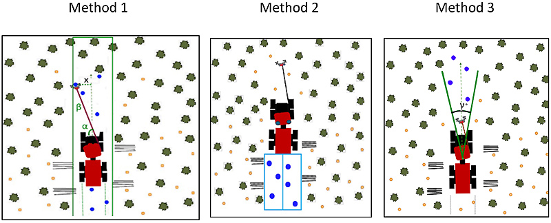
Fig. 1. Visualisation of the methods used to identify the strip-road trees.
Method 2 used the strip-road centreline as defined by the global coordinate system (Fig. 1). The harvester recorded its position each time a tree was fell-cut, and this information was used to reconstruct the strip road (Ovaskainen and Riekki 2022). A buffer was created around the computed centreline of the strip road, and the trees located within the buffer zone were classed as strip-road sample trees. To determine the effect of sample size, the widths of the buffer zone ranging from 1 to 6 m were tested in 0.5 m increments.
In Method 3, only the boom-angle information (γ) from the hpr data was used (Fig. 1). In this approach, the strip-road sample trees were identified within the boom sector ranging from 2 to 36°. The sector width was increased systematically in 2° increments. For each sector, the corresponding strip-road area was calculated to enable hectare-wise scaling. The strip-road sample area was computed as the product of the strip-road length and strip-road width. The strip-road width for each sector was derived trigonometrically using the maximum boom length and the corresponding sector angle, while the strip-road length was obtained from the computed strip-road based on the hpr data as in Method 2.
2.4 Spatial sensitivity of the strip-road sample
To address the second objective, within-stand variation was examined by establishing theoretical strip-road samples systematically across each stand. Straight lines were first generated at 20 m intervals across each stand, all oriented in the same main direction as the original strip-road network (Fig. 2). A 1.4 m buffer was applied on each side of the strip-road line to define a hypothetical strip-road width of 2.8 m, corresponding approximately to the width of the Komatsu 901XC-6 harvester. The trees of the pre-thinning treemap located within these buffered areas were extracted to represent the sample. The stem count and basal area were calculated for each strip-road area and then scaled to hectare-wise using the area of the sample. To compare these samples with the entire stand, each theoretical strip-road network was shifted by 1 m in the perpendicular direction. Assuming a strip-road spacing of 20 m, this shifting process was repeated 19 times to cover the full extent of the stand. This procedure enabled a systematic evaluation of how representative the individual strip-road samples were in relation to the entire stand. By comparing the variation across the parallel shifted strip-road networks, it was possible to assess the degree of spatial heterogeneity within the stands and to quantify the sampling sensitivity introduced by relying solely on the strip-road data.
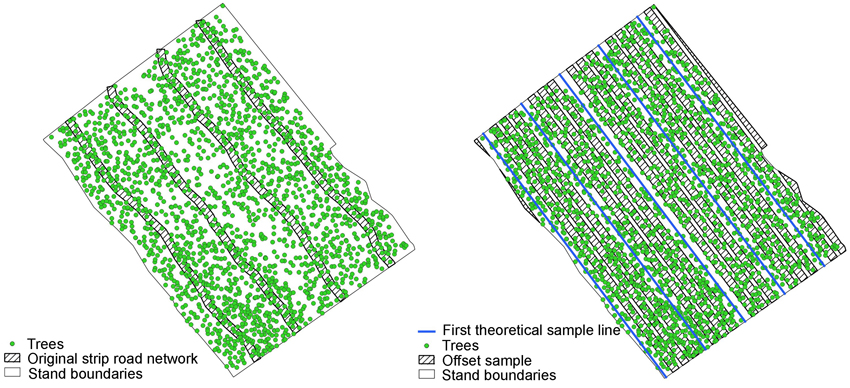
Fig. 2. Illustration of the original strip-road network (left figure) and three example offset sample networks from one stand (right figure). In total, 20 strip-road network positions were analysed stand-wise by shifting the network perpendicular to the strip-road direction in 1 m increments across the 20 m spacing.
By keeping the strip-road spacing, orientation and width constant while varying only the spatial phase of the network, the effect of spatial alignment from the other sources of variation was isolated. The resulting offset samples represented alternative realisations of the same deterministic sampling geometry and provided a means of evaluating the sensitivity of the strip-road-based estimates to the spatial heterogeneity within the stand.
2.5 Statistical methods
Reynold’s error index (REI), (Reynolds et al. 1988), was used to compare the estimated and reference distributions, calculated as follows:

where n is the index of the diameter class, N is the index of the largest diameter class in the datasets, gn is the basal area of the diameter class n, xn is the stem count of the diameter class n of the estimated distribution, and yn is the stem count of the diameter class n of the reference distribution. In interpreting the REI, lower values represent a good fit of the similarity of distributions. An absolute value of the difference of each class is weighted by the basal area, which reflects the correspondence of the distributions, especially at large diameters. Therefore, differences in large diameters affect the REI value more than differences in smaller diameters.
The root mean square error (RMSE) (Eq. 2) and relative RMSE were used to compare the different identification methods and sample sizes.

where  is the reference value,
  is the estimated value, and N is the number of observations.
3 Results
3.1 Strip-road tree identification methods
Across all seven measurement areas (A–G), there were clear differences among the tested strip road tree identification methods. Method 3 consistently produced higher REI values than the other two methods, indicating weaker correspondence with the reference diameter distributions. As the sector angle widened, the REI values increased steadily, reflecting the progressive inclusion of non-strip-road trees and distortion of the estimated diameter distribution. Only within a relatively narrow sector range (approximately 5–20° in two stands) the REI values fall below 10%, but this improvement was not consistent across the stands.
By contrast, both Methods 1 and 2 produced substantially lower REI values across most of the parameter ranges. The accuracy of Method 1 was strongly dependent on the selected strip-road width. When the selection width was narrow (0–2 meters), a portion of the actual strip-road trees remained unclassified, resulting in underestimation of the stem count and basal area. When the width increased beyond the effective machine width, the inclusion of thinning removals outside the strip road increased the REI values. An intermediate fixed range produced the lowest REI values, suggesting that correct geometric calibration is critical for this approach.
Method 2 demonstrated the most stable performance across the stands. By reconstructing the strip-road centrelines in a global coordinate system and applying a fixed-width buffer, this approach consistently produced low REI values and comparatively small relative RMSE values for the stem counts. Unlike in the sector-based approaches, the buffer method did not show systematic deterioration with moderate increases in buffer width. Instead, errors increased gradually once the buffer exceeded the actual operational strip-road width. This indicates that the spatially explicit representation of the strip-road width better captures the true geometry of the removals.
The relative RMSE comparisons across all stands (Fig. 3) further support these findings. The stem count RMSE% was the lowest for Methods 1 and 2 in most measurement areas, while Method 3 gave the largest deviations. Overall, the results show that incorporating spatial strip-road reconstructions substantially improves strip-road tree identification compared to method relying solely on crane-angle information.
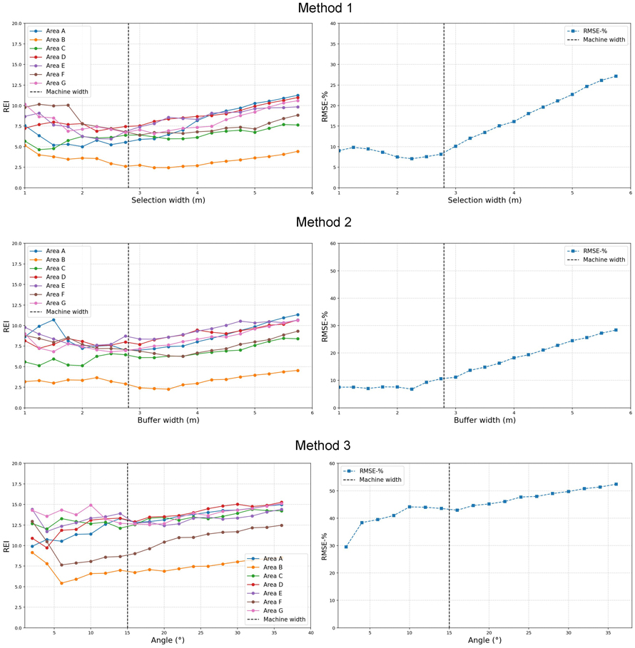
Fig. 3. Stand-wise REI values for each strip-road tree identification method and the relative RMSE values for all stands. View larger in new window/tab.
3.2 Spatial sensitivity of the strip-road sample
In addition to evaluating strip-road tree identification methods, the influence of strip-road placement on the representativeness of the sample was examined. The pre-harvest stem count references varied significantly across the seven measurement areas, ranging from 1250 to 1835 trees ha–1 (Table 1). In some measurement areas, the original strip-road samples closely matched the reference values (e.g. Area B, 1250 vs. 1199 trees ha–1), while in others, the difference was higher (e.g. Area A, 1718 vs. 1525 trees ha–1). The mean values of the offset samples generally aligned well with the reference data. Standard deviations of the offset samples ranged from 72 to 116 trees ha–1, indicating differences in sampling stability across the stands. The range between the minimum and maximum stem counts was more than 200 trees ha–1 for all measurement areas, the most being almost 400 in Area F.
| Table 1. Hectare-wise stem counts of the reference data, original strip-road samples and offset strip roads showing the standard deviations (std) and minimum and maximum stem counts of the offset strip-road samples. | |||||
| Measurement area | Reference stem count (n ha–1) | Original strip-road sample stem count (n ha–1) | Offset mean stem count (n ha–1) | Offset stem count std (n ha–1) | Offset min–max count (n ha–1) |
| A | 1718 | 1525 | 1714 | 82 | 1537–1817 |
| B | 1250 | 1199 | 1253 | 73 | 1152–1400 |
| C | 1717 | 1534 | 1649 | 72 | 1548–1828 |
| D | 1654 | 1524 | 1649 | 73 | 1438–1776 |
| E | 1404 | 1288 | 1414 | 74 | 1289–1528 |
| F | 1435 | 1328 | 1443 | 105 | 1218–1604 |
| G | 1835 | 1699 | 1846 | 116 | 1661–2080 |
The basal area estimates showed similar patterns (Table 2). The reference values ranged from 16.1 to 26.4 m2 ha–1, with the original strip-road samples underestimating the hectare-wise basal area. The offset samples typically deviated within ±0.2 m2 ha–1 from the reference, with standard deviations of between 1.2 and 2.2 m2 ha–1. There was an even higher difference in the minimum and maximum values. In five areas (Areas B, C and E–G), the difference was more than 5 m2. These results suggest that, while strip-road sampling can provide reasonable estimates, its accuracy is influenced by the local stand structure and the strip-road alignment.
| Table 2. Hectare-wise basal areas of the reference data, original strip-road samples and offset strip roads showing the standard deviations (std) and minimum and maximum basal areas of the offset strip-road samples. | |||||
| Measurement area | Reference basal area (m2 ha–1) | Original strip-road basal area (m2 ha–1) | Offset mean basal area (m2 ha–1) | Offset basal area std (m2 ha–1) | Offset min–max (m2 ha–1) |
| A | 24.5 | 19.8 | 24.7 | 1.2 | 21.5–27.1 |
| B | 16.1 | 14.5 | 16.1 | 1.5 | 13.6–18.8 |
| C | 24.7 | 20.4 | 24.5 | 1.7 | 21.4–26.2 |
| D | 24.7 | 19.3 | 24.6 | 1.2 | 21.1–27.0 |
| E | 23.7 | 18.5 | 23.9 | 1.3 | 21.4–26.4 |
| F | 22.0 | 19.0 | 22.1 | 2.2 | 18.2–26.8 |
| G | 26.4 | 21.7 | 26.5 | 1.8 | 22.4–29.8 |
Visualisations of the stem counts and basal areas across the offset samples (Fig. 4) highlight areas with higher internal variation, Areas F and G, in particular. In these stands, the standard deviations exceeded 100 trees ha–1 and 1.8 m2 ha–1, respectively, indicating that strip-road placement can significantly affect sample representativeness in particular stands. In all measurement areas, the stem count and basal area of the original strip road were lower than the reference and the offset average.
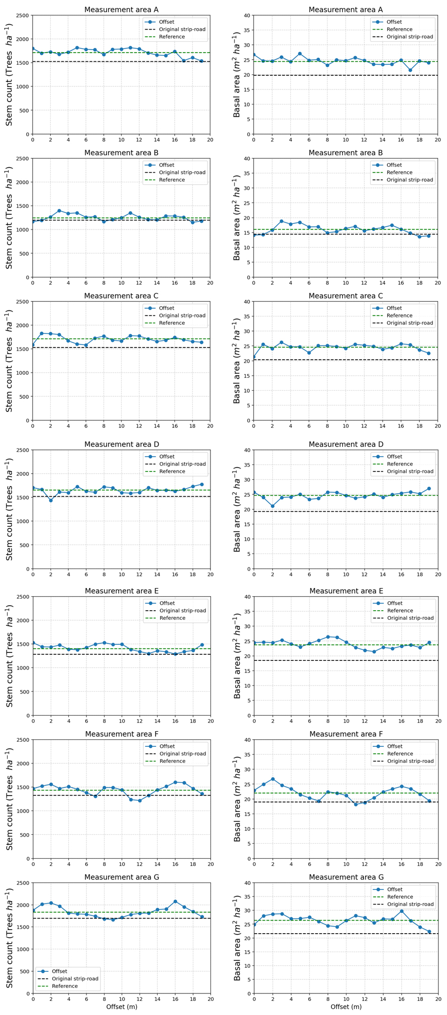
Fig. 4. Hectare-wise stem counts and basal areas for each offset sample (solid blue line with dots), reference value (green dashed line) and original strip-road sample (blue dashed line).
4 Discussion
The results show that strip-road sampling, based on harvester data from first thinnings, can provide a functional method for estimating pre-havest stand-level forest attributes, such as stem count and basal area. A key advantage of the approach is that it leverages information already collected during harvesting operations, making it both cost-effective and efficient compared with traditional field inventory data. Because strip roads typically cover 15–20% of the harvested area, the sample size is substantially larger than conventional plot-based inventories (Laasasenaho and Päivinen 1982; Haara and Leskinen 2009), which enhances the representativeness.
Among the three identification methods evaluated, Method 1 consistently produced the most accurate results, with lower REI and relative RMSE values for the stem count across all measurement areas. Method 1 has an advantage because its accuracy is not affected by global positioning. Method 2 also showed promising results. This suggests that incorporating spatial positioning data from the harvester, combined with a fixed-width buffer around the strip-road centreline, provides a reliable framework for identifying strip-road trees. However, Method 3 was less accurate, particularly as the sector angle increased, indicating that relying solely on the crane angle introduces greater uncertainty in tree identification.
The recent evaluation of hprGallring by Källmark (2025) is of relevance to the present study, as the underlying strip-road tree identification approach in hprGallring relies solely on boom angle (Bhuiyan et al. 2016; Möller et al. 2024), corresponding methodologically to Method 3 in our study. Notably, Källmark (2025) found that the strip-road width assumed by the software (4.3 m) underestimated the field-measured average width (4.6 m), Furthermore, the strip-road proportion estimated by hprGallring significantly exceeded field measurements by 12.2% on average, which the author attributed in part to this width assumption. These findings reinforce our conclusion that accurate calibration of strip-road geometry is critical for reliable strip-road-based sample identification.
From an operational perspective, the choice of strip-road tree identification method involves a trade-off between spatial precision and robustness to positioning uncertainty. However, the method’s performance is inherently dependent on GNSS accuracy and reliable reconstruction of the machine trajectory. By contrast, relying solely on the relative geometry between the machine and the felled tree makes it less sensitive to absolute positioning error.
There were limitations to the strip-road sampling. Strip-road placement is influenced by terrain, tree density and operational preferences, all of which can introduce bias. For example, operators may align strip roads with natural gaps or areas of smaller trees, leading to non-representative samples of strip-road trees. This was evident in the measurement areas F and G, where the offset samples showed substantial variation in stem count and basal area. In general, the stem count was closer to the reference and offset mean than the basal area, which might indicate that the strip roads were opened to areas with smaller trees. These findings underscore the importance of considering stand heterogeneity when interpreting strip-road data.
The offset strip sampling analysis demonstrated that, while the mean of the shifted strip-road samples closely approximated the reference, the individual realisations could deviate substantially in stands exhibiting pronounced spatial heterogeneity. This pattern indicates that strip-road sampling is not inherently biased at the stand level, but it is sensitive to spatial alignment relative to density gradients or structural clustering. It is also notable that all the original strip roads were positioned in areas of smaller trees and lower densities in the measurement areas, which raises concerns over the representativeness.
However, systematic sampling has always been exposed to design-based bias (Mandallaz 2008), especially when the starting point of the sampling is not random. Although strip roads form a regularly spaced line pattern, their placement does not satisfy the requirements of a probability-based systematic sample because the initial strip road is determined by operational and geographical constraints rather than randomisation. Instead, the offset analysis quantified the spatial sensitivity of the strip-road-derived estimates under alternative realisations of the same deterministic sampling geometry. From a model-based perspective, the influence of sampling geometry and spatial heterogeneity on estimation accuracy has been shown to be substantial, particularly in small-area applications (Kangas et al. 2025), which is consistent with the variability observed among the offset strip-road samples in this study.
In addition, the assumption of spatial homogeneity within stands may not always be true, particularly in mixed-species or uneven-aged forests. In such cases, strip-road samples may fail to capture the full variability of the stand, thus affecting the accuracy of upscaled estimates. Integrating complementary data sources, such as UAV imagery, LiDAR scans or pre-harvest inventory data, could help mitigate these limitations and improve the robustness of forest attribute estimation.
The empirical dataset consisted of seven measurement areas of approximately 1 ha each. Although the number of stands was limited, these areas represented the operational first-thinning conditions in western Finland and included the variations in stem density, basal area and spatial structure typical of managed boreal forests. The aim of this study was not to provide national-level inferences, but to evaluate methodological performance under realistic harvesting conditions. Nevertheless, broader validation across different site types, stand structures and geographical regions would be required before the findings can be generalised for operative use.
In Finland, field measurements of stand-level forest inventory is usually performed using a sample plot design that covers approximately 1–5% of the stand area. The accuracy of stand-level inventory varies due to the subjectivity of the sample plot placement, measurement errors and the experience of the measurer (Haara et al. 2009). Errors in the measurement of basal areas vary from about 10 to 22% (Laasasenaho and Päivinen 1986; Ståhl 1992). Errors in stem count inventory have not been investigated in Finland because the basal area is the main density metric, although in other Nordic studies, the stem count sample error is larger (Ståhl et al. 1992).
Research and industry have increasing interest in LiDAR technology to further enhance forest inventory capabilities e.g. measure DBH, stem curve and tree location for both removed and remaining trees. Ponsse’s Thinning Density Assistant (TDA) represents a commercially deployed example, using onboard LiDAR to provide real-time operator guidance on thinning density and strip-road spacing during first thinning (Pohjala et al. 2025). Such systems could directly address the key limitations identified in this study: they could provide an independent spatial reference for strip-road tree identification, reducing reliance on GNSS accuracy, and could measure the remaining stand directly rather than inferring it from the removed trees. However, integrating MLS data with hpr files poses non-trivial challenges. Tree species detection, errors and bias in DBH and other measurements, especially in younger stands, remains a challenging task for automated processes (Liikonen et al. 2026). Furthermore, Combining the high stem-level measurement accuracy of hpr data with the spatial completeness of MLS could ultimately yield a more robust inventory framework than either source alone.
Overall, strip-road sampling appears to be a promising tool for estimating forest inventory in thinning stands, but careful consideration of potential biases and the integration of complementary data sources, such as ALS or harvester mounted LiDAR measurements, could further strengthen its reliability. Strip-road sampling based on harvester data is a cost-efficient and dynamic approach for forest inventory in thinning stands.
5 Conclusions
Overall, harvester-based strip-road sampling offers a practical and cost-efficient alternative for forest inventory in thinning stands, benefiting from large sample sizes and data already having been collected during harvesting. However, the accuracy of the estimates depends strongly on the identification method used and on the spatial structure of the stand. Among the three evaluated identification approaches, the boom-angle and -length method produced the most reliable results across all measurement areas when carefully calibrated. The buffer-based method, which used reconstructed strip-road centrelines in a global coordinate system, provided acceptable results, albeit its performance was generally inferior to the buffer-based approach. Analysis of the theoretical, systematically shifted strip-road networks revealed notable within-stand variation in stem count and basal area in several stands. This indicates that strip-road samples are not always fully representative of the entire stand, particularly where spatial heterogeneity is pronounced or where the strip roads are preferentially aligned with gaps or smaller trees. Consequently, estimates based solely on realised strip-road locations may be biased in certain stand conditions. Future applications would benefit from incorporating adaptive strip-road widths, improved modelling of spatial heterogeneity and the integration of complementary data sources, such as ALS or harvester mounted LiDAR measurements, to further reduce bias and uncertainty.
Declaration of openness of research materials, data, and code
Restrictions apply to the availability of these data. The data is owned by stakeholders of Metsäteho Oy and is granted for the current purpose.
Authors’ contributions
Conceptualization (all); Methodology (R.T., H.O., K.R.); Software (R.T., H.O. and K.R.); Validation (R.T., K.R., and H.O.); Investigation (R.T., H.O. and K.R.); Data Curation (R.T., K.R.); Writing – Original Draft Preparation (R.T.); Writing – Review and Editing, (all); Visualization (R.T.); Supervision and Project Administration (J.M.); Funding Acquisition (J.M.) All authors have read and agreed to the published version of the manuscript.
Acknowledgements
We thank Metsäteho’s owners and their contractors for their excellent cooperation in collecting the data. Komatsu Forest AB is acknowledged for their assistance with the harvester data.
Funding of the research
This research has been conducted as a part of Ministry of Agriculture and Forestry program “Nappaa hiilestä kiinni” and as a part of project “Kestävän metsätalouden todentaminen ja menetelmät (KESTOTÄSMÄ)” funded by EU’s Recovery and Resilience Facility (RRF).
References
Bhuiyan N, Möller J J, Hannrup B, Arlinger J (2016) Automatisk gallringsuppföljning. Arealberäkning samt registrering av kranvinkel för identifiering av stickvägsträd och beräkning av gallringskvot. [Automatic follow-up of thinning. Stand area estimation and use of crane angle data to identify strip road trees and calculate thinning quotient]. Arbetsrapport 899, Skogforsk. https://www.skogforsk.se/cd_20190114161523/contentassets/6eda4307138347648171f87e3d9a3885/automatisk-gallringsuppfoljning-arealberakning-samt-registrering-av-kranvinkel-for-identifiering-av-sticktrad-och-berakning-av-gallringskvot-arbetsrapport-899-2016.pdf. Accessed 15 June 2026.
Brus D (2019) Sampling for digital soil mapping: a tutorial supported by R scripts. Geoderma 338: 464–480. https://doi.org/10.1016/j.geoderma.2018.07.036.
Cho H-M, Park J-W, Lee J-S, Han S-K (2024) Assessment of the GNSS-RTK for application in precision forest operations. Remote Sens 16, article id 148. https://doi.org/10.3390/rs16010148.
Cochran W (1977) Sampling techniques. Wiley, New York.
Flisberg P, Rönnqvist M, Willén E, Frisk M, Friberg G (2021) Spatial optimization of ground-based primary extraction routes using the BestWay decision support system. Can J For Res 51: 627–752. https://doi.org/10.1139/cjfr-2020-0238.
Haara A, Leskinen P (2009) The assessment of the uncertainty of updated stand-level inventory data. Silva Fenn 43: 87–112. https://doi.org/10.14214/sf.219.
Hannrup B, Möller J (2025) Test av förbättrad positionering i skördare. [Testing of improved positioning in a harvester]. Kunskapsartiklar 29-2025, Skogforsk. https://www.skogforsk.se/kunskapsbanken/kunskapsartiklar/2025/test-av-forbattrad-positionering-i-skordare/. Accessed 15 June 2026.
Isomäki A, Niemistö P (1990) Effect of strip roads on the growth and yield of young spruce stands in Southern Finland. Folia For 756: 1–36. https://urn.fi/URN:ISBN:951-40-1114-7.
Kaartinen H, Hyyppä J, Vastaranta M, Kukko A, Jaakkola A, Yu X, Pyörälä J, Liang X, Liu J, Wang Y, Kaijaluoto R, Melkas T, Holopainen M, Hyyppä H (2015) Accuracy of kinematic positioning using global satellite navigation systems under forest canopies. Forests 6: 3218–3236. https://doi.org/10.3390/f6093218.
Källmark E (2025) Utvärdering av hprGallring för automatisk gallringsuppföljning i barrskogar. Sveriges lantbruksuniversitet. Rapport från Institutionen för skogens biomaterial och teknologi 2025:8, Sveriges lantbruksuniversitet. http://urn.kb.se/resolve?urn=urn:nbn:se:slu:epsilon-s-21843.
Kangas A, Maltamo M (2006) Forest inventory. Methodology and applications. Springer, Dordrecht. https://doi.org/10.1007/1-4020-4381-3.
Kangas A, Astrup R, Breidenbach J, Fridman J, Gobakken T, Korhonen K, Maltamo M, Nilsson M, Nord-Larsen T, Næsset E, Olsson H (2018) Remote sensing and forest inventories in Nordic countries – roadmap for the future. Scand J For Res 33: 397–412. https://doi.org/10.1080/02827581.2017.1416666.
Kangas A, Myllymäki M, Packalen P (2025) The effect of sampling design in model-based small area estimation. Forestry 99, article id cpaf076. https://doi.org/10.1093/forestry/cpaf076.
Kärhä K, Kaartinen H, Backas J, Honkanen H, Hyyppä J, Hyyti H, Kankare V, Kinnunen V, Kukko A, Kymäläinen H, Laitinen J, Lopatin E, Pohjala J, Uro T, Vähä-Konka V, Väätäinen K (2025) Roadmap 2035 vision for forest machine data and sensor technologies. The future report produced by the IlmoStar Project. Publications of the University of Eastern Finland, Reports and Studies in Science, Forestry and Technology 10/2025. http://urn.fi/URN:ISBN:978-952-61-5717-7.
Laasasenaho J (1982) Taper curve and volume functions for pine, spruce and birch. Commun Inst For Fenn 108: 1–74. https://urn.fi/URN:ISBN:951-40-0589-9.
Laasasenaho J, Päivinen R (1982) On the checking of inventory by compartments. Folia For 664: 1–19. https://urn.fi/URN:ISBN:951-40-0757-3.
Liikonen L, Yrttimaa T, Erkkilä A, Paakkari J, Pitkänen T, Kotivuori E, Vastaranta M (2026) Measuring forest inventory attributes using Faro Orbis Mobile laser scanner in managed boreal forests. Forestry 99, article id cpag028. https://doi.org/10.1093/forestry/cpag028.
Lindroos O, Ringdahl O, La Hera P, Hohnloser P, Hellström T (2015) Estimating the position of the harvester head – a key step towards the precision forestry of the future? Croat J For Eng 36: 147–164.
Mandallaz D (2008) Sampling techniques for forest inventories. Chapman and Hall/CRC, London. https://doi.org/10.1201/9781584889779.
Möller JJ, Bhuiyan N, Arlinger J, Eriksson I, Söderberg J, Hannrup B (2024) hprYield – beräkningsmodul för generering av geografiskt uppdelade nyckeltal baserade på skördardata. Arbetsrapport 1228–2024. Skogforsk, Uppsala. https://www.skogforsk.se/contentassets/2d0af30a469b4500b5cf61cef2ad4ca6/arbetsrapport-1228-2024-hpryield--berakningsmodul-for-generering-av-geografiskt-uppdelade-nyckeltal-baserade-pa-skordardata.pdf. Accessed 15 June 2026.
Myllymäki M, Tuominen S, Kuronen M, Packalen P, Kangas A (2024) The relationship between forest structure and naturalness in the Finnish national forest inventory. Forestry 97: 339–348. https://doi.org/10.1093/forestry/cpad053.
Natural Resources Institute Finland Statistics Database (2026) https://statdb.luke.fi/PxWeb/sq/616db989-d7ff-4e97-bff4-19b934a98ff2. Accessed 13 August 2026.
Ovaskainen H, Riekki K (2022) Computation of strip road networks based on harvester location data. Forests 13, article id 782. https://doi.org/10.3390/f13050782.
Pohjala J, Kankare V, Hyyppä J, Kärhä K (2025) Effects of a mobile LiDAR-based thinning density assistant (TDA) system on harvester operator performance. Eur J For Res 144: 1301–1322. https://doi.org/10.1007/s10342-025-01808-y.
Pukkala T (1990) A method for incorporating the within-stand variation into forest management planning. Scand J For Res 5: 263–275. https://doi.org/10.1080/02827589009382611.
QGIS.org (2025) QGIS Geographic Information System. QGIS Association. http://www.qgis.org.
Reynolds M, Burk T, Huang W (1988) Goodness-of-fit tests and model selection procedures for diameter distribution models. For Sci 34: 373–399. https://doi.org/10.1093/forestscience/34.2.373.
Sagar A, Pohjala J, Muhojoki J, Dhital A, Kaartinen H, Kärhä K, Järvelin K, Ghabcheloo R, Hyyppä J, Kankare V (2026) Utilising mobile laser scanning point clouds to assess harvesting quality in thinning stands. Sci Remote Sens 13, article id 100374. https://doi.org/10.1016/j.srs.2026.100374.
Skogforsk (2025) StanForD/StanForD 2010 standard for forest machine data and communication. http://www.skogforsk.se/english/projects/stanford. Accessed 15 June 2026.
Ståhl G (1992) En studie av kvalitet i skogliga avdelningsdata som insamlats med subjektiva inventerigsmetoder. [Summary of a study on the quality of compartment-wise forest data acquired by subjective inventory methods]. Rapport 24, Swedish University of Agricultural Sciences.
Tarvainen R, Riekki K, Ovaskainen H, Poikela A, Kärhä K, Malinen J (2025) Estimating stand variables in first-thinnings using harvester data. Silva Fenn 59, article id 25014. https://doi.org/10.14214/sf.25014.
Total of 31 references.
Send to email

