Sakari Tuominen  ,
Timo Pitkänen,
Andras Balazs,
Annika Kangas
,
Timo Pitkänen,
Andras Balazs,
Annika Kangas
Improving Finnish Multi-Source National Forest Inventory by 3D aerial imaging
Tuominen S., Pitkänen T., Balazs A., Kangas A. (2017). Improving Finnish Multi-Source National Forest Inventory by 3D aerial imaging. Silva Fennica vol. 51 no. 4 article id 7743. https://doi.org/10.14214/sf.7743
Highlights
- 3D aerial imaging provides a feasible method for estimating forest variables in the form of thematic maps in large area inventories
- Photogrammetric 3D data based on aerial imagery that was originally acquired for orthomosaic production was tested in estimating stand variables
- Photogrammetric 3D data highly improved the accuracy of forest estimates compared to traditional 2D remote sensing imagery.
Abstract
Optical 2D remote sensing techniques such as aerial photographing and satellite imaging have been used in forest inventory for a long time. During the last 15 years, airborne laser scanning (ALS) has been adopted in many countries for the estimation of forest attributes at stand and sub-stand levels. Compared to optical remote sensing data sources, ALS data are particularly well-suited for the estimation of forest attributes related to the physical dimensions of trees due to its 3D information. Similar to ALS, it is possible to derive a 3D forest canopy model based on aerial imagery using digital aerial photogrammetry. In this study, we compared the accuracy and spatial characteristics of 2D satellite and aerial imagery as well as 3D ALS and photogrammetric remote sensing data in the estimation of forest inventory variables using k-NN imputation and 2469 National Forest Inventory (NFI) sample plots in a study area covering approximately 5800 km2. Both 2D data were very close to each other in terms of accuracy, as were both the 3D materials. On the other hand, the difference between the 2D and 3D materials was very clear. The 3D data produce a map where the hotspots of volume, for instance, are much clearer than with 2D remote sensing imagery. The spatial correlation in the map produced with 2D data shows a lower short-range correlation, but the correlations approach the same level after 200 meters. The difference may be of importance, for instance, when analyzing the efficiency of different sampling designs and when estimating harvesting potential.
Keywords
forest inventory;
remote sensing;
spatial autocorrelation;
spatial distribution;
aerial imagery;
stereo-photogrammetry
-
Tuominen,
Natural Resources Institute Finland (Luke), Economics and Society, P.O. Box 2, FI-00791 Helsinki, Finland
E-mail
sakari.tuominen@luke.fi
- Pitkänen, Natural Resources Institute Finland (Luke), Economics and Society, P.O. Box 2, FI-00791 Helsinki, Finland E-mail timo.p.pitkanen@luke.fi
- Balazs, Natural Resources Institute Finland (Luke), Economics and Society, P.O. Box 2, FI-00791 Helsinki, Finland E-mail andras.balazs@luke.fi
- Kangas, Natural Resources Institute Finland (Luke), Economics and Society, P.O. Box 68, FI-80101 Joensuu, Finland E-mail Annika.Kangas@luke.fi
Received 5 June 2017 Accepted 31 July 2017 Published 16 August 2017
Views 151545
Available at https://doi.org/10.14214/sf.7743 | Download PDF

1 Introduction
Satellite imagery (such as Landsat or SPOT XS imagery) has been used in remote sensing-aided forest inventories for a long time to produce geospatial estimates of forest characteristics. A successful example of this is the Finnish multi-source National Forest Inventory (MS-NFI) (Tomppo 1993; Tomppo et al. 2008). Starting from the late 1980s, MS-NFI has been used operationally for producing forest information in the form of thematic forest maps and forest statistics for municipal areas.
The MS-NFI method is based on combining information from field sample plots of National Forest Inventory (NFI), satellite images and digital map data. In general, the satellite images enable covering larger areas but have considerably lower spatial resolution compared to aerial images. On the other hand, they cover wider spectral variation and generally enable more feasible operational use due to their frequent acquisition and public distribution at no cost (Roy et al. 2014; Barrett et al. 2016). The main drawback is that the general accuracy of satellite image-based forest estimates is not sufficient for forest management purposes at the forest stand level.
Aerial imagery can be used both in management-oriented forest inventories (Köhl 1993; Pekkarinen and Tuominen 2003) and in NFIs (Poso 1972; Keller 2001). Compared to satellite imagery such as Landsat, the higher spatial resolution of aerial imagery allows the use of textural image features in addition to spectral information (Woodcock and Strahler 1987; Lillesand et al. 2004). Better resolution, together with textural features, help to recognize small-scale variations and horizontal vegetation structure in more detail (Wood et al. 2012), therefore improving the estimates of stand-level forest attributes (Poso et al. 1999). The availability and affordability of aerial images is generally good in Finland, and the recently established national aerial imaging program ensures further updates at maximum five years’ interval for almost the whole country (Tuominen and Pekkarinen 2005; Maltamo et al. 2006; Maanmittauslaitos 2016).
During the last 15 years, airborne laser scanning (ALS) has been adopted in many countries including Finland for the estimation of forest attributes at stand and sub-stand levels. Compared to optical remote sensing data sources, ALS data are particularly well-suited for the estimation of forest attributes related to the physical dimensions of trees, such as stand height and volume, due to the three-dimensional (3D) nature of the data (van Aardt et al. 2006; Yu et al. 2011; Kankare et al. 2013). In forestry use, ALS data is typically summarized using a rasterized grid, where each grid cell is populated with a range of ALS-derived metrics and further applied in model development (Wulder et al. 2012). ALS is currently considered to be the most accurate remote sensing method for estimating stand-level forest variables (Næsset 2002, 2004; Maltamo et al. 2004; Bergseng et al. 2015; Wilkes et al. 2015; White et al. 2016). On the other hand, with the pulse densities applied in operational forest inventories, ALS is not considered to be well-suited for estimating tree species composition or dominance and, thus, optical imagery is typically acquired to complement the ALS data (Törmä 2000; Waser et al. 2011; Fassnacht et al. 2016). Due to the high cost of ALS data, it is usually not a feasible method for covering large areas with good temporal resolution (Barrett et al. 2016).
Similar to ALS, it is possible to derive a 3D forest canopy surface model (CSM) based on aerial imagery using digital aerial photogrammetry (Pitt et al. 2014; Stepper et al. 2016). This requires imagery with sufficiently high spatial resolution and stereo overlap. 3D CSMs derived from aerial photographs using stereo-photogrammetric measurement have been reported to be well correlated to CSMs generated from ALS data, and they can be considered as a viable alternative to ALS (Baltsavias et al. 2008; Pitt et al. 2014), although their geometric accuracy is often lower (St-Onge et al. 2008; Haala et al. 2010). The main benefit of the photogrammetric canopy model is that no separate flights are required for the acquisition of 3D data and imagery, which often have different flight parameters in relation to the imaging altitude and coverage in case of ALS and aerial imagery. Furthermore, aerial images are typically acquired at frequent intervals for purposes other than forestry such as mapping and surveying, which increases their availability compared to ALS data (Granholm et al. 2015; Stepper et al. 2016). Therefore, aerial images have significant potential for operational use in forestry applications (Bohlin et al. 2012).
In this study we examine the stereo-photogrammetric 3D canopy data derived from archived aerial imagery as a potential data source covering the requirements of large area forest inventory (aiming at high area coverage) while simultaneously serving the needs of management-oriented forest inventory (aiming at high local accuracy). The primary focus of this paper is on large area inventory compatible with the results of current operational MS-NFI. In particular, we focus on an approach where traditional 2D aerial and satellite image data are complemented with 3D CSM derived from aerial stereo-imagery. The forest estimates based on stereo-photogrammetric 3D CSM are compared to those based on traditional 2D remote sensing data, as well as to the estimates based on ALS data and aerial orthoimagery.
2 Materials and methods
2.1 Study area
The study area is located in central Finland and covers approximately 5800 km² (Fig. 1). The topography of the area is relatively flat with elevation values ranging generally between 100–200 m above sea level. A majority of the region is characterized by oligotrophic moraine and peat soil deposits. These areas have traditionally been unfavorable for settlement and cultivation, and they have mainly been allocated for forestry. Thus, the study area is characterized by a wide coverage of forested areas, sparse inhabitation and lack of significant urban areas. In addition, the area is part of the Suomenselkä watershed zone which separates two drainage basins, one having streams running towards the Gulf of Bothnia (west) and the other towards the Gulf of Finland (south).
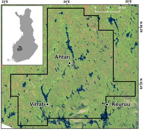
Fig. 1. Study area in Finland visualized on top of the Landsat 8 image (2014) used in the study.
The study area belongs predominantly to the middle boreal vegetation zone with some southern boreal influences in its southern parts. According to 2013 Finnish multi-source NFI results, 78.8% of the total area (470 000 ha) is used for forestry purposes, while the remaining coverage is primarily dominated by a few larger water bodies and scattered agricultural areas. Of the forestry land, 72.0% is mineral soil, 26.2% forested peatland and 1.8% open bogs or mires. Forests are mainly coniferous and dominated by Scots pine (Pinus sylvestris L.; 54.1%), Norway spruce (Picea abies [L.] H. Karst.; 5.4%), or by combination of the two (21.8%). To a lesser extent, there are also mixed forests (7.4%), broadleaved forests (mainly Betula pendula Roth and B. pubescens Ehrh.; 4.9%) and sparsely forested areas (6.5%). The principal silvicultural system in the region has been even-aged management.
2.2 Field data
A total of 2469 sample plots were placed on the study area using systematic cluster sampling. Each of the full clusters had eight plots with 250 m spacing in two orthogonal rows, and clusters were placed 4.3 km apart from each other both horizontally and vertically (Tomppo et al. 2016) (Fig. 2). Clusters at the edges of the study area contained less than eight sample plots. Of the 2469 defined plots, 1956 (79.2%) were located on forestry land.
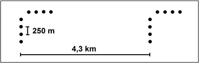
Fig. 2. Field sampling design used in the study.
All trees whose diameter at breast height (dbh, in our case, diameter at the height of 1.3 m) was at least 4.5 cm were calipered for a fixed radius plot of 9 m. Tree species, dbh, tree class, distance from the center point of a plot to the tree, as well as the azimuth of the tree, were recorded for all tally trees. The distance and azimuth were measured simultaneously with the Masser Sonar caliper. Additionally, the average age and height of the trees were measured from the basal area median trees of each tree species group. Additionally, a small set of stand-level characteristics were measured from each stand intersecting a plot (Tomppo et al. 2016).
The statistics of the most important forest variables, measured from the plots located on forestry land, are presented in Table 1. In addition, the distribution of volume classes is illustrated in Fig. 3.
| Table 1. Field-measured mean, standard deviation (SD) and maximum (Max) values of tree height (H) and diameter at breast height (D) as well as volume metrics including pine, spruce and broadleaved species. | ||||||
| H (m) | D (cm) | Vol tot (m3 ha–1) | Vol pine (m3 ha–1) | Vol spruce (m3 ha–1) | Vol Broadl. (m3 ha–1) | |
| Mean | 12.7 | 15.6 | 120.9 | 73.3 | 28.5 | 19.1 |
| SD | 5.83 | 7.54 | 95.6 | 70.8 | 63.4 | 34.3 |
| Max | 28.1 | 43.8 | 867.3 | 519.9 | 461.3 | 411.9 |
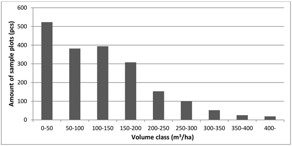
Fig. 3. Distribution of total tree volume in the sample plots.
2.3 Remote sensing data
Aerial images used in the study were digitally acquired in good weather conditions during July and August in 2013. Imagery was acquired using a Microsoft UltraCam Eagle camera, and the imaging altitude was 4700 m. Images contained red (R), green (G), blue (B) and near-infrared (NIR) spectral bands, and they were orthorectified to a ground resolution of 30 cm per pixel. Furthermore, based on the photogrammetric measurements of stereo pair images, a 3D point cloud (canopy surface model, CSM) representing the uppermost canopy layer was calculated using Trimble MATCH-T software. This point cloud covers the study area in the form of an evenly spaced grid with 0.75 m intervals between points (excluding water bodies).
Since the operational MS-NFI of Finland is based on using satellite imagery as remote sensing data source, we used Landsat satellite image as a point of comparison. Landsat 8 images were used both for comparison and for complementing the information based on aerial images with satellite data. As no suitable Landsat 8 materials were available from summer 2013, a frame acquired on July 23rd, 2014 was downloaded from United States Geological Survey (USGS) service as an atmospherically corrected surface reflectance product (see Fig. 1). To replace patches affected by clouds or their shadows, a second surface reflectance Landsat 8 frame, acquired on July 3rd, 2015, was downloaded as well. Both of the images were carefully rectified using aerial images, band-wise reflectance histograms of the 2015 image were matched to the 2014 image, and finally cloudy/shadowy patches of 2014 were replaced with the data of 2015. In this study, bands 1–7 were used.
The second reference remote sensing method used in this study for comparison was a combination of ALS and aerial imagery, used in forest inventories aiming at producing stand-level forest data for forest management. ALS data were acquired originally for the Finnish Forest Centre in June–August 2013 using an Optech Gemini ALTM laser scanner. The scanning altitude was 1730 m with a maximum zenith angle of 20° and side overlap of 20%. The average density of points in the ALS point cloud was 0.91 m–2, strip overlap was 20%, half scan angle 20 degrees and the maximum number of observed pulse returns was four. Both the digital terrain model (DTM) and canopy surface model (CSM) were derived from ALS data. Pulse returns with heights greater than 1.3 m above the ground were classified as canopy. The DTM was produced in two phases (Tomppo et al. 2016). In the first phase the area was divided into 8 × 8 m grid cells and each grid cell’s ground elevation was calculated using the average elevation above sea level of the ground points inside the grid cell if there were at least three ground points. For grid cells with less than three ground points the elevation was calculated in the second phase using neighboring cells with ground elevation values and a Gaussian weighing function. The height above ground (H) was calculated for each LiDAR point as the difference between the z coordinate and the estimated ground level.
A digital terrain model was provided by the open data file download service of the National Land Survey of Finland (National Land Survey 2017). Approximately 75% of the study area was covered by a terrain model based on ALS data and generated at 2 m pixel size, while the remaining 25% had been constructed earlier using aerial images at 10 m pixel size. The terrain model was applied with photogrammetric point cloud data for determining the terrain elevation in relation to photogrammetric point cloud. This DTM was not available at the time when ALS data was processed. As with ALS, canopy height (above ground) was calculated for each point of the photogrammetric 3D data.
3 Methods
3.1 Extraction of remote-sensing features
Canopy height values of the photogrammetric point cloud were interpolated into a raster format canopy height model (CHM) at spatial resolution and grid spacing similar to that of the digital aerial images. Final height values were limited to between 0and 40 m, thus covering the expected variation in the forests of the study area and reducing the effects of potential outliers.
Remote sensing features for sample plots were extracted from the ALS point clouds, photogrammetric point clouds, the rasterized canopy height model (derived from the photogrammetric point data) as well as from the aerial and satellite images.
Features extracted from ALS and aerial image data sets for a different study (Tomppo et al. 2016) were used and are described in that article.
Raster features were extracted from 16 × 16 m square windows, whose centers coincided with the centers of the sample plots. Features from the photogrammetric point data were extracted from around the sample plots’ centers within a radius of 9 m.
The following features were extracted from the photogrammetric point data (Næsset 2002; Maltamo et al. 2009):
1. Average value of H for vegetation points (m)
2. Standard deviation of H for vegetation points (m)
3. H at which percentiles of vegetation points (0%, 5%, 10%, 20%, ..., 85%, 90%, 95%, 100%) accumulated (m)
4. Coefficient of variation of H for vegetation points (%)
5. Proportion of vegetation points relative to all points (%)
6. Proportions of vegetation points having H above fraction* 0, 1, ..., 9 from all points (%)
7. Ratio of the number of vegetation points to the number of ground points
8. Proportion of ground points (%)
* The range of H was divided into 10 fractions (0, 1, 2, …, 9), of equal distance.
where H = return/point height above ground
vegetation return/point = return/point with H ≥ 1.3 m
ground return/point = other than vegetation return/point
The following features were extracted from the CSMs:
1. Averages of pixel values
2. Standard deviations of pixel values
3. Textural features based on co-occurrence matrices of pixel values (Haralick et al. 1973; Haralick 1979):
• Angular Second Moment
• Contrast
• Correlation
• Variance
• Inverse Difference Moment
• Sum Average
• Sum Variance
• Sum Entropy
• Entropy
• Difference Variance
• Difference Entropy
• Information Measures of Correlation 1
• Information Measures of Correlation 2
The textural features based on co-occurrence matrices of pixel values were extracted as average values for features calculated in four directions in the extraction window: horizontally (0° angle), vertically (90°), and diagonally (45° and 135°). The same set of textural features was extracted from aerial images with a pixel lag of 2.7 meters additionally to the lag of 5.7 meters used by Tomppo et al. (2016).
The following features were extracted from the satellite image:
1. Pixel values in each image band
2. Ratios of all possible band combinations (excluding reciprocals)
3. Normalized difference vegetation index (NDVI), 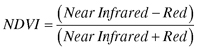
4. NDVIGreen, 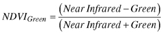
Single pixel values from the sample plot centers were extracted.
All features were scaled to have a standard deviation of 1. This was done because the original features had very diverse scales of variation. Without scaling, variables with wide variation would have had greater weight in the estimation regardless of their correlation with the estimated forest attributes.
3.2 Estimation of forest attributes and selection of remote-sensing features
The k-nearest neighbor (k-NN) method was used for the estimation of the forest variables. Different values of k (3–6) were tested in the estimation procedure. The nearest neighbors were weighted by the inverse squared Euclidean distances for diminishing the averaging of the estimates (Altman 1992). The following Euclidean distance d was applied in k-NN (Eq. 1):

where pj is the pixel j, p is the target pixel, fl is the l th feature, wl is the weight of l th feature. The weight of sample plot I to pixel p was defined as:

where N is the neighborhood of k nearest sample plots i1(p)…ik(p) of pixel p. Then, a pixel-level estimate for variable y is:
![]()
The selection of the features (as well as the optimal value of k) was performed with a genetic algorithm (GA)-based approach, implemented in the R language by means of the Genalg package (Willighagen and Ballings 2015; R Development Core Team 2016). Here the evaluation function of the genetic algorithm was employed to minimize the root mean square errors (RMSE) (Eq. 4) of the k-NN estimates of inventory variables in leave-one-out cross-validation. In cross-validation the estimated forest variable values were compared with the measured values (ground truth) of the sample plots.
where M is the number of sample plots. The relative RMSE was obtained by relating the RMSE to the mean value of the variable in question.
3.3 Distribution of forest attribute estimates
In addition to cross-validating the estimates, the amount of variation (of field data) that can be retained in the estimates was examined. The distribution histograms of the field data, operational MS-NFI (from year 2013), and the method combining satellite images and aerial photos (2D and 3D) (hereafter referred as 3D-MS-NFI) were calculated for volumes of growing stock (both total and for tree species groups pine, spruce and broadleaved trees) as well as for mean height. K-NN estimation method typically cannot extrapolate estimate values outside the reference values, and it also often causes undesirable averaging in the estimates, especially in the higher end of growing stock volume. This is partly due to the fact that the assortment of potential reference plots with a large volume or tree size is often limited. The averaging is more pronounced when the correlation between inventory variables and remote sensing features is low. For example, spectral features of satellite imagery typically have a poor ability to discriminate forests with volumes greater than 250 m3 ha–1. Furthermore, the value of k affects the amount of original variation (of field observations) that can be retained in the estimates; the higher the value of k the more averaging occurs.
3.4 The spatial distribution and autocorrelation
Spatial structure and local autocorrelation of the operational MS-NFI data and 3D-MS-NFI predictions were also visualized using correlograms (Fig. 8). A correlogram indicates autocorrelation values which are plotted against distances among localities, given the expectations that there is a certain dominant spatial structure found in the study area, and this structure is isotropic i.e. independent of the observation direction (Legendre and Fortin 1989). Correlogram calculations used in this study are based on a nonparametric spline-derived technique described by Bjørnstad and Falck (2001) and implemented in R statistical software using the “ncf” package. Correlograms are closely related to semivariograms but offer a standardized range from –1 to +1 rather than a magnitude-dependent variance measure, thus allowing an easier comparison between the different data sets and regions (Legendre and Fortin 1989; Meisel and Turner 1998; Overmars et al. 2003). Due to the heavy calculation routines related to correlogram determination, a 2.5 × 2.5 km analysis window was selected from the middle of the study area which was expected to represent the spatial structure of the total study area.
4 Results
4.1 Accuracy of forest variables
In the estimation of the total volume of growing stock, satellite image spectral features resulted in a relative RMSE of 60.95%, which was slightly better than the combination of spectral and textural features (i.e. “traditional” 2D image features) of aerial orthoimagery (RMSE 62.45%). When combining the aforementioned satellite and aerial image features, the accuracy of volume estimates was 57.66%, i.e. somewhat better than the estimates that resulted from any of those data sources separately. A major improvement in the estimation accuracy was achieved only when 3D point cloud features were introduced. The combination of ALS and 2D aerial image features (as used in management-oriented forest inventory) resulted in the best volume estimation accuracy (RMSE 27.80%), but there was no large difference in the accuracy compared to estimates based on photogrammetric 3D data in combination with satellite and/or aerial image features. Here the inclusion of satellite image features with point cloud features resulted in slightly better accuracy (RMSE 31.26%) than aerial image features (RMSE 31.53%). The RMSE of the total volume estimates using stereo-photogrammetric 3D data was approx. 11% larger than that produced with ALS.
When estimating volumes per tree species groups (pine, spruce and deciduous trees) the trend and the order of the tested data sources was almost exactly similar, with the main exception that the aerial image 2D features performed better than satellite image features here. Furthermore, the inclusion of the satellite image data with the combination of aerial image 2D data and photogrammetric 3D data made a more pronounced difference in the volume estimates per tree species (compared to total volume estimates). The estimation accuracy of the total growing stock volume and volumes per tree species groups with the tested data combinations is illustrated in Fig. 4.
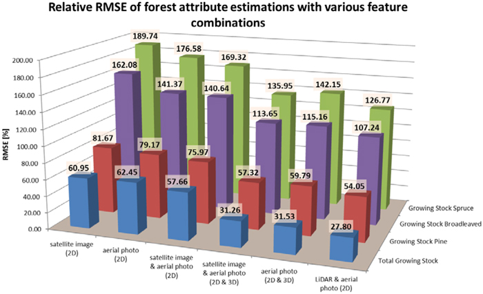
Fig. 4. Relative RMSEs of volume (total, pine, broadleaved trees and spruce) estimates.
In the estimation of basal area the relative accuracy of the estimates with the tested data combinations were almost in proportion to those of total volume estimates, and the order of the tested data sources was similar. When estimating forest variables directly related to the size of the trees, i.e. mean height and diameter, there was a clear difference in the performance of 2D satellite and aerial image features. Here, aerial imagery performed somewhat better than satellite features, and combining them did not bring marked improvement compared to aerial image features only. For the estimates of mean height and diameter the inclusion of 3D features brought much greater improvement in the accuracy than for growing stock volumes (total or per tree species). Thus, the poorest estimates of height and diameter were based on satellite image features, RMSE 33.78 and 37.50%, respectively. Aerial image 2D features gave RMSEs of 31.16% for height and 34.23% for diameter, and the combination of satellite and aerial images 29.93% for height and 33.27% for diameter. Inclusion of aerial (stereo-photogrammetric) 3D features with satellite image features reduced the RMSEs of height and diameter estimates to 11.49% and 17.02%, respectively, and combining satellite data with aerial image 2D and 3D features resulted in RMSEs of 10.99% for height and 17.14% for diameter. Again, the best estimates were based on combination of ALS 3D data and aerial 2D features, but the difference between ALS and stereo-photogrammetric 3D data was clearly smaller here than in the case of volume. Here the difference in the accuracy of the best estimates using ALS or stereo-photogrammetric 3D data was only 4.8% for height and 1.7% for diameter. The estimation accuracy of the basal area, height and diameter with the tested data combinations is illustrated in Fig. 5.
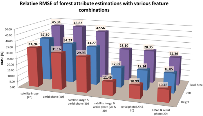
Fig. 5. Relative RMSEs of height, DBH and basal area estimates.
4.2 Distributions of forest variables
As a general tendency, sample plots gain higher frequencies at both ends of the distributions compared to operational MS-NFI and 3D-MS-NFI predictions (i.e. satellite images and aerial photos 2D and 3D), which are more prone to predict values relatively close to the variable mean (Fig. 6). Of these two methods, however, 3D-MS-NFI frequencies are generally closer to the field-derived data. This tendency is particularly evident with total volume of the growing stock. Correct estimates of extremely high values seem to be problematic for both MS-NFI and 3D-MS-NFI methods, although the latter is closer to the field-measured values with all the measured variables.
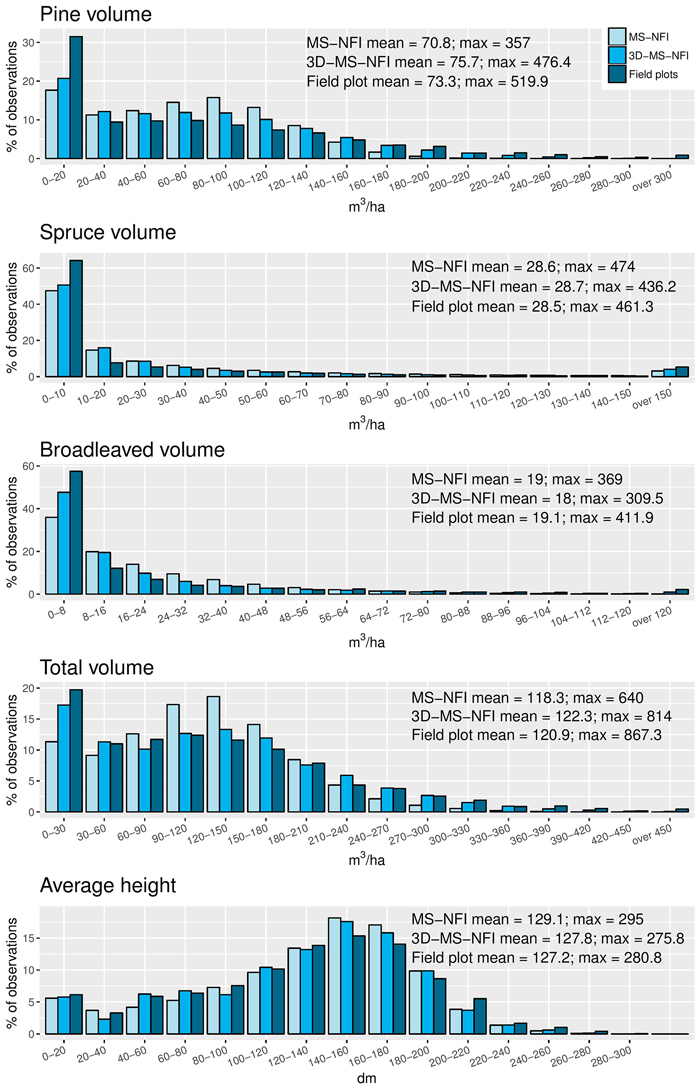
Fig. 6. Histograms of the different variables from operational MS-NFI, 3D-MS-NFI results (satellite image and aerial photos 2D + 3D) of this study, and sample plots. Features selected for this comparison are total volumes of growing stock for pine, spruce and broadleaved trees, and average height of the trees.
Mean values of MS-NFI, 3D-MS-NFI and field data are relatively similar to each other. In terms of maximum values, 3D-MS-NFI mean is always lower compared to the field data, but MS-NFI values exceed the field data with spruce volume and average height. Based on the histograms, these differences appear to be due to single pixels rather than reflecting general emphasis on higher values. It must be also noticed that although all the data are targeted at representing the same area and year, operationally produced MS-NFI data is based on a different set of sample plots compared to the ones used in the 3D-MS-NFI calculations, and there are also differences in the used satellite images. Mimicking the whole operational chain within this study in order to use the same field data, however, would have been complicated and expectedly led to similar results compared to the applied MS-NFI data.
4.3 Spatial configuration of the forest area
In Fig. 7, volumes of growing stock and average height have been visualized using a small subsection of the study area. The figure indicates clear differences in the spatial structure between the MS-NFI and 3D-MS-NFI estimates. In particular, values predicted by the operational MS-NFI method tend to be less extreme and more scattered compared to the 3D-MS-NFI values, which appear to construct larger continuous patches. In addition, border lines between the dissimilar patches are visually more distinctive with 3D-MS-NFI data than with MS-NFI predictions.
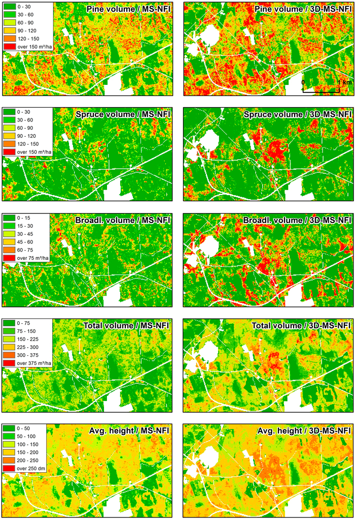
Fig. 7. Visualization of the different variables based on operational MS-NFI (left) and 3D-MS-NFI results of this study (right) related to growing stock volumes and average height.
In the correlograms presented in Fig. 8, the 3D-MS-NFI curve starts generally from a higher initial correlation and remains above the MS-NFI values until at least a 200 m distance. This stands for higher similarity of the variable values at close distances, i.e. indicating stronger spatial autocorrelation and the existence of larger relatively homogeneous patches. In forest estimates based on satellite imagery, high proportion of pixels are mixed (i.e. receive reflectance from more than one stand) due to the small average stand size, approx. 1–2 ha in Southern Finland (Tokola and Kilpeläinen 1999; Mäkelä and Pekkarinen 2001). When using higher resolution remote sensing data, the landscape patch structure is more evident in mapped data (proportion of mixed pixels is lower). At approximately 200–300 m distance, autocorrelation levels out close to zero level. The only exceptional curve is the spruce volume. However, one should notice that spruce is not the dominant tree species and the study area is rather characterized by relatively low mean volume and comparatively high standard deviation (Table 1).
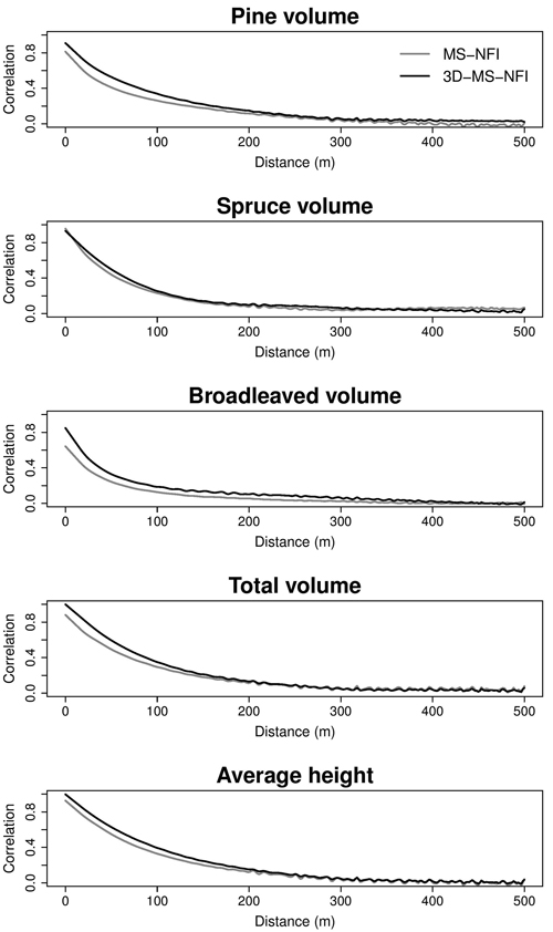
Fig. 8. Correlograms (i.e. correlation as a function of distance between pixels) of the growing stock volumes (pine, spruce, broadleaved, total) and average height.
5 Discussion
In this study, the inclusion of 3D information to complement 2D data resulted in a major enhancement in estimation accuracy. Depending on the variable, the difference in RMSEs could be close to 100%. On the other hand, the differences between 3D materials from ALS and photogrammetric point clouds were much smaller, albeit still clear. Although the photogrammetric point cloud appears to be a very crude representation of the canopy structure (Fig. 9), there is strikingly little difference between key features extracted from photogrammetric and ALS point clouds, for example, in relation to stand height (Fig. 10). The importance of this difference in decision making remains to be studied, for instance with a cost-plus-loss analysis (Bergseng et al. 2015).
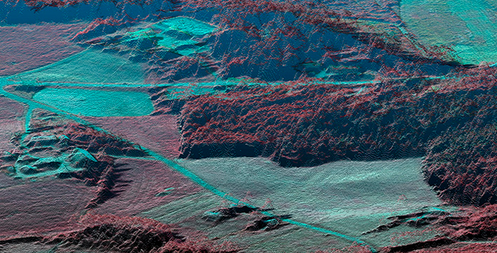
Fig. 9. An illustration of the photogrammetric point cloud.
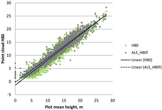
Fig. 10. Scatter plot describing the relation of H80 feature of 3D cloud points (first points only in ALS data) vs. measured value (H80 was selected because it usually corresponds well to the mean height of a plot). Linear trendline of ALS data shows R2 = 0.9405; with photogrammetric data R2 = 0.9203.
The possibility of collecting data during relatively frequent aerial image acquisition campaigns, however, improves the operational feasibility and cost efficiency of CSMs compared to ALS data. Whether standard image acquisition parameters are sufficient for CSM production, particularly related to image overlap, has been a recent topic of discussion. Puliti et al. (2017) and Bohlin et al. (2012), for example, tested and compared overlaps of both 60% and 80%. Puliti et al. (2017) found 80% overlap slightly outperforms 60%, but Bohlin et al. (2012) reported to have detected no improvement from higher overlap. This may result from a trade-off between increased image matching success when using higher overlap, and simultaneous decrease in height accuracy due to a shorter baseline between the images leading to weaker relief displacement (Lemaire 2008). 60% overlap was used in this study, which also corresponds to the Finnish image acquisition standards. In addition to ALS and CSM data, 3D information can be retrieved by radar data from spaceborne platforms such as TanDEM-X or TerraSAR-X as well as very high resolution (VHR) optical satellites. Radar materials are able provide a more generalized mid-canopy response, but gained accuracy remains generally at a lower level compared to airborne sources (Wulder et al. 2012; Rahlf et al. 2014; Yu et al. 2015). VHR-derived 3D data, in turn, may produce results which are comparable or even outperform the CSMs created from aerial images (Yu et al. 2015; Stone et al. 2016), but the current costs of acquiring VHR materials over large coverages for the needs of operational use may turn out to be unacceptable. Furthermore, it should be stressed that all the methods except ALS are relying on the existence of good quality ground elevation models, which may pose restrictions to the selection of the applicable method.
The differences between the spaceborne and airborne 2D data were mixed; in some cases spaceborne data was more accurate than airborne data, and vice versa. This indicates that the wide spectral range of multispectral satellite imagery still has advantages over the high spatial resolution of aerial imagery. As their combined use leads to an augmented range of available features, including wider spectral and textural variation, it is however slightly surprising that the model including both aerial photos and satellite images does not result in more distinctive improvement compared to the single-data models. This could potentially be explained by mixed signals given by the two data sources due to their different initial resolutions, particularly referring to the coarser resolution of the Landsat data (30 m) compared to the analysis window used in this study (16 × 16 m). In addition, the applied Landsat frame was from one year later compared to the aerial images and field data, thus adding a potential source of errors to the analysis.
The relative RMSEs of total volume for the 3D material here were markedly higher than in Puliti et al. (2017), namely 31.60 for image matching data and 27.80 for ALS, compared to 21.3 and 19.7 in Puliti et al. (2017), respectively. One obvious reason for this difference is that the mean volume in this study was 120 m3, while in Puliti et al. (2017) it was 248.3 m3. In this study, all forest development classes were included, while in the study of Puliti et al. (2017) young stands and recently regenerated or open areas were left out. A respective difference can also be seen in the species-level results. Furthermore, several studies have reported that the use of ALS data markedly outperforms photogrammetrically created point clouds in forest variable estimation. Rahlf et al. (2014), for example, found that ALS resulted in a 19% RMSE at the plot-level compared to 31% RMSE for photogrammetric data. Similar results have also been obtained by Vastaranta et al. (2013), where the RMSEs for total volume were 18% and 25% for ALS and photogrammetric point clouds, respectively and Järnstedt et al. 2012, with 31% and 40%, and with Straub et al. (2013) with 34% and 41%. Generally the differences between these two methods have thus been clear. It is possible that these differences are related to the ALS point density, which in the abovementioned studies ranged between 5 and 10 pulses m–2, while the density used in this study was less than one point per square meter and footprint size was larger due to higher flight altitude. However, the resolutions of the aerial images and CSMs generated from them were also differing and there were variations in the fieldwork planning and data collection, therefore making it difficult to define any single reason for the observed differences. These examples nevertheless indicate that ALS has capabilities in accurate forest variable estimation, but from the perspective of repetitive large area operational analyses aiming at frequently updated products similar to the present MS-NFI, requiring relatively frequent and repetitive estimations over large areas, production of high-density ALS data may not be a feasible option.
The effect of adding 3D information to support 2D information is clearly seen from the histograms of the forest variables, and from the spatial distribution as well. When using k-NN-based estimation, it is often unavoidable that distribution tails near to minimum and maximum values of the reference data are partially neglected as k observations are used to calculate the estimates. A closer match of the 3D-MS-NFI distribution with field data compared to the operational MS-NFI values, however, proves that 3D information can clearly improve the accuracy of estimates over a larger range of values. This could further lead to better success in forest type classification, particularly emphasizing the detection of those classes, which without 3D data would be underrepresented (Dalponte et al. 2008). In terms of spatial structure, more distinctive border lines created by the 3D-MS-NFI data have a closer match to reality, given the current forestry system in Finland which favors periodical clearcuts, often followed by planting a single species and resulting in even-aged stand structure (Kuuluvainen et al. 2012). The support of 3D data may be explained by its capabilities to measure more directly variables such as forest volume, DBH, basal area and particularly average height, whereas the sole use of 2D data primarily offers correlating surrogates to indicate these characteristics. Surrogates are beneficial in measuring variables that would otherwise be difficult to interpret, such as using image texture to reflect the actual physical canopy composition (Wulder 1998), but more direct variables will normally increase the accuracy of the results.
The forest resource maps produced with satellite images have often also been used for optimizing the sampling design (Tomppo et al. 2011). When selecting the cluster size and the distances of plots within the cluster, autocorrelation is very important. The map estimated using satellite images has lower autocorrelation than the 3D-MS-NFI map utilizing point cloud data especially in the range of 200 meters, but the difference is negligible with larger distances. This indicates that while both of the data types are able to detect similar characteristics in terms of general forest structure, the 3D-MS-NFI version with added 3D information is more prone to generate smaller homogeneous patches, which is reflected by increased spatial autocorrelation at short distances. Such a tendency is likely to improve the detection of stand-related forest structures, and further lead to, e.g., easier identification of harvesting opportunities. The importance of this difference from the decision making point of view still needs to be examined.
Acknowledgements
The authors wish to thank Ministry of Agriculture and Forestry key project "Puuta liikkeelle ja uusia tuotteita metsästä" for the financial support for this study
References
Altman N.S. (1992). An introduction to kernel and nearest-neighbor nonparametric regression. The American Statistician 46(3): 175–185. https://doi.org/10.1080/00031305.1992.10475879.
Baltsavias E., Gruen A., Eisenbeiss H., Zhang L., Waser L.T. (2008). High-quality image matching and automated generation of 3D tree models. International Journal of Remote Sensing 29(5): 1243–1259. https://doi.org/10.1080/01431160701736513.
Barrett F., McRoberts R.E., Tomppo E., Cienciala E., Waser L.T. (2016). A questionnaire-based review of the operational use of remotely sensed data by national forest inventories. Remote Sensing of Environment 174: 279–289. https://doi.org/10.1016/j.rse.2015.08.029.
Bergseng E., Ørka H.O., Næsset E., Gobakken T. (2015). Assessing forest inventory information obtained from different inventory approaches and remote sensing data sources. Annals of Forest Science 72(1): 33–45. https://doi.org/10.1007/s13595-014-0389-x.
Bjørnstad O.N., Falck W. (2001). Nonparametric spatial covariance functions: estimation and testing. Environmental and Ecological Statistics 8(1): 53–70. https://doi.org/10.1023/A:1009601932481.
Bohlin J., Wallerman J., Fransson J.E.S. (2012). Forest variable estimation using photogrammetric matching of digital aerial images in combination with a high-resolution DEM. Scandinavian Journal of Forest Research 27(7): 692–699. https://doi.org/10.1080/02827581.2012.686625.
Dalponte M., Bruzzone L., Gianelle D. (2008). Fusion of hyperspectral and LIDAR remote sensing data for classification of complex forest areas. IEEE Transactions on Geoscience and Remote Sensing 46(5): 1416–1427. https://doi.org/10.1109/TGRS.2008.916480.
Fassnacht F.E., Latifi H., Stereńczak K., Modzelewska A., Lefsky M., Waser L.T., Straub C., Ghosh A. (2016). Review of studies on tree species classification from remotely sensed data. Remote Sens. Environ 186: 64–87. https://doi.org/10.1016/j.rse.2016.08.013.
Granholm A.-H., Olsson H., Nilsson M., Allard A., Holmgren J. (2015). The potential of digital surface models based on aerial images for automated vegetation mapping. International Journal of Remote Sensing 36(7): 1855–1870. https://doi.org/10.1080/01431161.2015.1029094.
Haala N., Hastedt H., Wolf K., Ressl C., Baltrusch S. (2010). Digital photogrammetric camera evaluation – generation of digital elevation models. Photogrammetrie - Fernerkundung - Geoinformation 2010(2): 99–115. https://doi.org/10.1127/1432-8364/2010/0043.
Haralick R.M. (1979). Statistical and structural approaches to texture. Proceedings of the IEEE 67(5): 786–804. https://doi.org/10.1109/PROC.1979.11328.
Haralick R.M., Shanmugam K., Dinstein I. (1973). Textural Features for Image Classification. IEEE Transactions on Systems, Man, and Cybernetics SMC-3(6): 610–621. https://doi.org/10.1109/TSMC.1973.4309314.
Järnstedt J., Pekkarinen A., Tuominen S., Ginzler C., Holopainen M., Viitala R. (2012). Forest variable estimation using a high-resolution digital surface model. ISPRS Journal of Photogrammetry and Remote Sensing 74: 78–84. https://doi.org/10.1016/j.isprsjprs.2012.08.006.
Kankare V., Vastaranta M., Holopainen M., Räty M., Yu X., Hyyppä J., Hyyppä H., Alho P., Viitala R. (2013). Retrieval of forest aboveground biomass and stem volume with airborne scanning LiDAR. Remote Sensing 5(5): 2257–2274. https://doi.org/10.3390/rs5052257.
Kuuluvainen T., Tahvonen O., Aakala T. (2012). Even-aged and uneven-aged forest management in boreal fennoscandia: a review. Ambio 41(7): 720–737. https://doi.org/10.1007/s13280-012-0289-y.
Legendre P., Fortin M.J. (1989). Spatial pattern and ecological analysis. Vegetatio 80(2): 107–138. https://doi.org/10.1007/BF00048036.
Lemaire C. (2008). Aspects of the DSM production with high resolution images. In: Proceedings of the XXI ISPRS Congress, 3 Jul 2008, Beijing, China. p. 1143–1146.
Lillesand T.M., Kiefer R.W., Chipman J.W. (2004). Remote Sensing and Image Interpretation (5th ed.). John Wiley and Sons Inc, New York, NY, USA.
Maanmittauslaitos (2016). Kansallinen ilmakuvausohjelma käynnistyy. http://www.maanmittauslaitos.fi/ajankohtaista/kansallinen-ilmakuvausohjelma-kaynnistyy. [Cited 2 Jun 2017].
Mäkelä H., Pekkarinen A. (2001). Estimation of timber volume at the sample plot level by means of image segmentation and Landsat TM imagery. Remote Sensing of Environment 77(1): 66–75. https://doi.org/10.1016/S0034-4257(01)00194-8.
Maltamo M., Eerikäinen K., Pitkänen J., Hyyppä J., Vehmas M. (2004). Estimation of timber volume and stem density based on scanning laser altimetry and expected tree size distribution functions. Remote Sensing of Environment 90(3): 319–330. https://doi.org/10.1016/j.rse.2004.01.006.
Maltamo M., Malinen J., Packalén P., Suvanto A., Kangas J. (2006). Nonparametric estimation of stem volume using airborne laser scanning, aerial photography, and stand-register data. Canadian Journal of Forest Research 36(2): 426–436. https://doi.org/10.1139/x05-246.
Maltamo M., Packalén P., Suvanto A., Korhonen K.T., Mehtätalo L., Hyvönen P. (2009). Combining ALS and NFI training data for forest management planning: a case study in Kuortane, Western Finland. European Journal of Forest Research 128(3): 305–317. https://doi.org/10.1007/s10342-009-0266-6.
Meisel J.E., Turner M.G. (1998). Scale detection in real and artificial landscapes using semivariance analysis. Landscape Ecology 13(6): 347–362. https://doi.org/10.1023/A:1008065627847.
Næsset E. (2002). Predicting forest stand characteristics with airborne scanning laser using a practical two-stage procedure and field data. Remote Sensing of Environment 80(1): 88–99. https://doi.org/10.1016/S0034-4257(01)00290-5.
Næsset E. (2004). Accuracy of forest inventory using airborne laser scanning: evaluating the first nordic full-scale operational project. Scandinavian Journal of Forest Research 19(6): 554–557. https://doi.org/10.1080/02827580410019544.
Overmars K.P., de Koning G.H.J., Veldkamp A. (2003). Spatial autocorrelation in multi-scale land use models. Ecological Modelling 164(2–3): 257–270. https://doi.org/10.1016/S0304-3800(03)00070-X.
Pekkarinen A., Tuominen S. (2003). Stratification of a forest area for multisource forest inventory by means of aerial photographs and image segmentation. In: Corona P., Kfhl M., Marchetti M. (eds.). Advances in forest inventory for sustainable forest management and biodiversity monitoring. Forestry Sciences 76:111–123. https://doi.org/10.1007/978-94-017-0649-0_9.
Pitt D.G., Woods M., Penner M. (2014). A comparison of point clouds derived from stereo imagery and airborne laser scanning for the area-based estimation of forest inventory attributes in boreal Ontario. Canadian Journal of Remote Sensing 40(3): 214–232. https://doi.org/10.1080/07038992.2014.958420.
Puliti S., Gobakken T., Ørka H.O., Næsset E. (2017). Assessing 3D point clouds from aerial photographs for species-specific forest inventories. Scandinavian Journal of Forest Research 32(1): 68-79. https://doi.org/10.1080/02827581.2016.1186727.
R Development Core Team (2016). R: a language and environment for statistical computing. Vienna, Austria. http://www.r-project.org. [Cited 2 March 2017].
Rahlf J., Breidenbach J., Solberg S., Næsset E., Astrup R. (2014). Comparison of four types of 3D data for timber volume estimation. Remote Sensing of Environment 155: 325–333. https://doi.org/10.1016/j.rse.2014.08.036.
Roy D.P., Wulder M.A., Loveland T.R., Woodcock C.E., Allen R.G., Anderson M.C., Helder D., Irons J.R., Johnson D.M., Kennedy R., Scambos T.A., Schaaf C.B., Schott J.R., Sheng Y., Vermote E.F., Belward A.S., Bindschadler R., Cohen W.B., Gao F., Hipple J.D., Hostert P., Huntington J., Justice C.O., Kilic A., Kovalskyy V., Lee Z.P., Lymburner L., Masek J.G., McCorkel J., Shuai Y., Trezza R., Vogelmann J., Wynne R.H., Zhu Z. (2014). Landsat-8: science and product vision for terrestrial global change research. Remote Sensing of Environment 145: 154–172. https://doi.org/10.1016/j.rse.2014.02.001.
St-Onge B., Vega C., Fournier R.A., Hu Y. (2008). Mapping canopy height using a combination of digital stereo-photogrammetry and lidar. International Journal of Remote Sensing 29(11): 3343–3364. https://doi.org/10.1080/01431160701469040.
Stepper C., Straub C., Immitzer M., Pretzsch H. (2016). Using canopy heights from digital aerial photogrammetry to enable spatial transfer of forest attribute models: a case study in central Europe. Scandinavian Journal of Forest Research 1–14. https://doi.org/10.1080/02827581.2016.1261935.
Stone C., Webster M., Osborn J., Iqbal I. (2016). Alternatives to LiDAR-derived canopy height models for softwood plantations: a review and example using photogrammetry. Australian Forestry 79(4): 271–282. https://doi.org/10.1080/00049158.2016.1241134.
Straub C., Stepper C., Seitz R., Waser L.T. (2013). Potential of UltraCamX stereo images for estimating timber volume and basal area at the plot level in mixed European forests. Canadian Journal of Forest Research 43(8): 731–741. https://doi.org//10.1139/cjfr-2013-0125.
Tokola T., Kilpeläinen P. (1999). The forest stand margin area in the interpretation of growing stock using Landsat TM imagery. Canadian Journal of Forest Research 29(3): 303–309. https://doi.org/10.1139/x98-200.
Tomppo E. (1993). Multi-source national forest inventory of Finland. In: Nyyssönen A., Poso S., Rautala J. (eds.). Proceedings of Ilvessalo Symposium on National Forest Inventories, 17–21 Aug. 1992, Finland. The Finnish Forest Research Institute Research Papers 444: 52–60.
Tomppo E., Haakana M., Katila M., Peräsaari J. (2008). Multi-source national forest inventory – methods and applications. Managing Forest Ecosystems 18. Springer. 374 p.
Tomppo E., Heikkinen J., Henttonen H.M., Ihalainen A., Katila M., Mäkelä H., Tuomainen T., Vainikainen N. (2011). Designing and conducting a forest inventory – case: 9th National Forest Inventory of Finland (Vol. 22). Springer, Dordrecht. https://doi.org/10.1007/978-94-007-1652-0_1.
Tomppo E., Kuusinen N., Mäkisara K., Katila M., McRoberts R.E. (2016). Effects of field plot configurations on the uncertainties of ALS-assisted forest resource estimates. Scandinavian Journal of Forest Research 1–13. https://doi.org/10.1080/02827581.2016.1259425.
Törmä M. (2000). Estimation of tree species proportions of forest stands using laser scanning. International Archives of Photogrammetry and Remote Sensing 33(Part B7): 1524–1531.
Tuominen S., Pekkarinen A. (2005). Performance of different spectral and textural aerial photograph features in multi-source forest inventory. Remote Sensing of Environment 94(2): 256–268. https://doi.org/10.1016/j.rse.2004.10.001.
van Aardt J.A.N., Wynne R.H., Oderwald R.G. (2006). Forest volume and biomass estimation using small-footprint lidar-distributional parameters on a per-segment basis. Forest Science 52(6): 636–649.
Vastaranta M., Wulder M.A., White J.C., Pekkarinen A., Tuominen S., Ginzler C., Kankare V., Holopainen M., Hyyppä J., Hyyppä H. (2013). Airborne laser scanning and digital stereo imagery measures of forest structure: comparative results and implications to forest mapping and inventory update. Canadian Journal of Remote Sensing 39(5): 382–395. https://doi.org/10.5589/m13-046.
Waser L.T., Ginzler C., Kuechler M., Baltsavias E., Hurni L. (2011). Semi-automatic classification of tree species in different forest ecosystems by spectral and geometric variables derived from Airborne Digital Sensor (ADS40) and RC30 data. Remote Sensing of Environment 115(1): 76–85. https://doi.org/10.1016/j.rse.2010.08.006.
White J.C., Coops N.C., Wulder M.A., Vastaranta M., Hilker T., Tompalski P. (2016). Remote sensing technologies for enhancing forest inventories: a review. Canadian Journal of Remote Sensing 42(5): 61–641. https://doi.org/10.1080/07038992.2016.1207484.
Wilkes P., Jones S.D., Suarez L., Haywood A., Woodgate W., Soto-Berelov M., Mellor A., Skidmore A.K. (2015). Understanding the effects of ALS pulse density for metric retrieval across diverse forest types. Photogrammetric Engineering and Remote Sensing 81(8): 33–43. https://doi.org/10.14358/PERS.81.8.625.
Willighagen E., Ballings M. (2015). genalg: R based genetic algorithm. https://cran.r-project.org/web/packages/genalg/index.html. [Cited 2 March 2017].
Wood E.M., Pidgeon A.M., Radeloff V.C., Keuler N.S. (2012). Image texture as a remotely sensed measure of vegetation structure. Remote Sensing of Environment 121: 516–526. https://doi.org/10.1016/j.rse.2012.01.003.
Woodcock C.E., Strahler A.H. (1987). The factor of scale in remote sensing. Remote Sensing of Environment 21(3): 311–332. https://doi.org/10.1016/0034-4257(87)90015-0.
Wulder M.A., White J.C., Nelson R.F., Næsset E., Ørka H.O., Coops N.C., Hilker T., Bater C.W., Gobakken T. (2012). Lidar sampling for large-area forest characterization: a review. Remote Sensing of Environment 121: 196–209. https://doi.org/10.1016/j.rse.2012.02.001.
Yu X., Hyyppä J., Vastaranta M., Holopainen M., Viitala R. (2011). Predicting individual tree attributes from airborne laser point clouds based on the random forests technique. ISPRS Journal of Photogrammetry and Remote Sensing 66(1): 28–37. https://doi.org/10.1016/j.isprsjprs.2010.08.003.
Yu X., Hyyppä J., Karjalainen M., Nurminen K., Karila K., Vastaranta M., Kankare V., Kaartinen H., Holopainen M., Honkavaara E., Kukko A., Jaakkola A., Liang X., Wang Y., Hyyppä H., Katoh M. (2015). Comparison of laser and stereo optical, SAR and InSAR point clouds from air- and space-borne sources in the retrieval of forest inventory attributes. Remote Sensing 7(12): 15933–15954. https://doi.org/10.3390/rs71215809.
Total of 55 references.
