Matti Maltamo  ,
Marius Hauglin,
Erik Naesset,
Terje Gobakken
,
Marius Hauglin,
Erik Naesset,
Terje Gobakken
Estimating stand level stem diameter distribution utilizing harvester data and airborne laser scanning
Maltamo M., Hauglin M., Naesset E., Gobakken T. (2019). Estimating stand level stem diameter distribution utilizing harvester data and airborne laser scanning. Silva Fennica vol. 53 no. 3 article id 10075. https://doi.org/10.14214/sf.10075
Highlights
- Tree level-positioned harvester data were successfully used as plot-level training data for k-nearest neighbor stem diameter distribution modelling applying airborne laser scanning information as predictor variables
- Stand-level validation showed that merchantable volume of total tree stock could be estimated with RMSE value of about 9%
- The fit of the stem diameter distribution assessed by a variant of Reynold’s error index showed values smaller than 0.2
- The most accurate results were obtained for the training plot sizes of 200 m2 and 400 m2.
Abstract
Accurately positioned single-tree data obtained from a cut-to-length harvester were used as training harvester plot data for k-nearest neighbor (k-nn) stem diameter distribution modelling applying airborne laser scanning (ALS) information as predictor variables. Part of the same harvester data were also used for stand-level validation where the validation units were stands including all the harvester plots on a systematic grid located within each individual stand. In the validation all harvester plots within a stand and also the neighboring stands located closer than 200 m were excluded from the training data when predicting for plots of a particular stand. We further compared different training harvester plot sizes, namely 200 m2, 400 m2, 900 m2 and 1600 m2. Due to this setup the number of considered stands and the areas within the stands varied between the different harvester plot sizes. Our data were from final fellings in Akershus County in Norway and consisted of altogether 47 stands dominated by Norway spruce. We also had ALS data from the area. We concentrated on estimating characteristics of Norway spruce but due to the k-nn approach, species-wise estimates and stand totals as a sum over species were considered as well. The results showed that in the most accurate cases stand-level merchantable total volume could be estimated with RMSE values smaller than 9% of the mean. This value can be considered as highly accurate. Also the fit of the stem diameter distribution assessed by a variant of Reynold’s error index showed values smaller than 0.2 which are superior to those found in the previous studies. The differences between harvester plot sizes were generally small, showing most accurate results for the training harvester plot sizes 200 m2 and 400 m2.
Keywords
LIDAR;
cut-to length harvester;
GPS;
merchantable volume;
tree list
-
Maltamo,
University of Eastern Finland, School of Forest Sciences, P.O. Box 111, FI-80101 Joensuu
E-mail
matti.maltamo@uef.fi
- Hauglin, Norwegian Institute of Bioeconomy Research, Division of Forest and Forest Resources, P.O. Box 115, 1431 Ås, Norway E-mail marius.hauglin@nibio.no
- Naesset, Norwegian University of Life Sciences, Faculty of Environmental Sciences and Natural Resource Management, P.O. Box 5003, 1432 Ås, Norway E-mail erik.naesset@nmbu.no
- Gobakken, Norwegian University of Life Sciences, Faculty of Environmental Sciences and Natural Resource Management, P.O. Box 5003, 1432 Ås, Norway E-mail terje.gobakken@nmbu.no
Received 20 November 2018 Accepted 5 August 2019 Published 7 August 2019
Views 76336
Available at https://doi.org/10.14214/sf.10075 | Download PDF

Supplementary Files
1 Introduction
The use of airborne laser scanning (ALS) for forest inventories has been growing over the past 15 years (Næsset 2014; White et al. 2013). This is due to the high level of accuracy of estimated forest attributes and continuously reduced acquisition costs of the remotely sensed data caused by the rapid development of the laser scanner technology. In forestry, laser scanning applications are usually related to forest management inventories where rather large inventory areas are covered wall-to-wall by ALS data and then subsequently divided into management units (Næsset 2014; Maltamo and Packalen 2014). Alternatively, ALS data have also been used as a sample of auxiliary data in large-area inventories where the ALS survey is designed according to probabilistic principles (Ståhl et al. 2011). The use of field training data is inevitable in all types of ALS-based forest inventories to construct models relating stand attributes to remote sensing metrics. Usually the data acquisition costs of field data represent a substantial part of the overall inventory costs due to laborious field work. Numerous efforts have been made to reduce costs of field data acquisition. These include, for example, use of existing plots from previous inventories (Kotivuori et al. 2018) and more effective use of the field plot data by applying properties of the ALS data as prior information when selecting locations of the field plots to be measured in field (Hawbaker et al. 2009), which is a topic related to model-based sampling.
Another option to reduce field data acquisition costs is to utilize field data acquired primarily for other purposes. Some studies have examined the usability of national forest inventory (NFI) plots as training data (Maltamo et al. 2009b; Tuominen et al. 2014; Nilsson et al. 2017) for management inventories. In general, the results are promising and for example Nilsson et al. (2017) have constructed nationwide forest attribute maps for Sweden using ALS and NFI plots. However, lack of precise plot positioning, inhomogeneous plot types and sizes and small sampling intensity have limited the usability of NFI plots in management inventories.
Data collected for other purposes than forest inventory may also be a viable alternative to establish training data. It has, for example, been proposed to use tree level cut-to-length harvester data collected in forest operations (Bollandsås et al. 2011). Harvester data are collected during harvesting from each stem to be cut. The data include a large number of diameter measurements along the stem and usually cover all merchantable timber in clear-cut stands, except retention trees.
In earlier studies, harvester data have been used as for example a stem data bank when planning future forest operations (Malinen et al. 2001), for mapping forest yield (Olivera and Visser 2016) or to generate field data for logged stands (Rasinmäki and Melkas 2005). Harvesters are equipped with an autonomous global navigation satellite system (GNSS) receiver which registers the location of the harvester body. Such positional data offer only low accuracy for single-tree locations. According to Lindroos et al. (2015) the error is typically in the range of 10–20 m. Harvester data have nevertheless been related to ALS data to predict or validate estimates of forest attributes. Bollandsås et al. (2011) demonstrated such a methodology for relatively large estimation units (0.25 ha) and Peuhkurinen et al. (2008) and Siipilehto et al. (2017) validated ALS-based predictions using a stem data bank at stand level. Some other studies have used manually positioned tree-level field data in combination with ALS and harvester data (Holmgren et al. 2012; Barth and Holmgren 2013).
Recently, Hauglin et al. (2017, 2018) showed that tree-level positioned harvester data with a mean positional error of < 1 m are obtainable using GNSS and real time kinematic (RTK) positioning. Hauglin et al. (2018) applied four different statistical modelling methods to compare predictions of plot-level volume when the ALS-based models were calibrated either by accurately positioned harvester data or using manually measured field plot data. The results showed that comparable accuracies were obtained with the two methods.
Stem diameter distribution is one of the main attributes to characterize the forest resources in many countries. The distribution is needed for the calculation of stand timber assortments and it also reflects the silvicultural state and allows simulation of the future development of a forest stand using single-tree growth models. Estimation of stem diameter distribution has been a research topic using both cut-to-length harvester data (Malinen et al. 2001) and for ALS data (Gobakken and Næsset 2004; Shang et al. 2017). The relationship between the stem diameter distribution and the ALS metrics typically computed from ALS point clouds have been found to be strong (Maltamo et al. 2018) but the small sizes of inventory plots may have a negative influence the accuracy of stem diameter distributions estimated from ALS. The accuracy is also lower for species-specific estimates, especially for minor tree species (Packalén and Maltamo 2008). When considering species-specific estimates of stem diameter distributions, the use of non-parametric techniques such as nearest neighbor imputation have been attractive because of the ability to provide simultaneous prediction of all attributes of interest (Packalén and Maltamo 2008; Räty al. 2018).
Effects of plot size have been assessed in previous studies (e.g. Gobakken and Næsset 2008). In mature forests, effects of plot sizes of 200 and 400 m2 have been compared. When constructing stand attribute (mean height, basal area and volume) regression models fitted to ALS-derived metrics, it was revealed that the model error in most cases was smaller for larger plots while the coefficient of correlation tended to be larger (Gobakken and Næsset 2008). Additionally, Næsset et al. (2011) applied design-based, model-assisted estimators with ALS data to estimate the biomass in a forest inventory and compared different plot sizes and found larger plots to result in smaller standard errors of estimates. These findings indicate that larger field plots may be favorable in forest inventories assisted by ALS.
Another issue related to field sample plots is the sampling intensity within each stand. While modelling usually has been done with smaller plots due to the large field measurement costs of larger plots, the validation of the models has been performed with larger plots or with stands for which reference estimates have been based on many plots sampled within each stand (Holmgren 2004; Næsset 2007; Packalén and Maltamo 2008). Use of larger validation units has improved the validation accuracy but still the area of the plots/stands used for validation is rather small compared to operational stand sizes. For example in Finland, the average stand size is around two hectares and the minimum 0.5 hectares (Koivuniemi and Korhonen 2006).
The overall aim of the current study was to examine the accuracy of stand stem diameter distributions estimated by utilizing accurately positioned single-tree data from a harvester and ALS metrics as predictor variables by nearest neighbor imputation. We focused on the dominant tree species, Norway spruce, but due to the flexible properties of the applied estimation methods, all species and stand totals were considered as well. We also evaluated effects of different plot sizes ranging from 200 m2 to 1600 m2 and validated the estimates at stand level which consisted of all plots located within a stand. Validated stand attributes included stand total basal area, number of stems, and merchantable volumes by species and in total. In addition, mean diameter, merchantable volume of saw-log sized trees and diameter percentiles of Norway spruce were considered. All the analyzed attributes can be calculated from tree lists. The study data is the same as in Hauglin et al. (2018).
2 Materials and methods
The study area was located in the Romerike region in Akershus County, Norway (60°25´N, 11°04´E, 200–600 m above sea level, Fig. 1). The forests in Romerike are boreal and dominated by Norway spruce (Picea abies (L.) H. Karst.) and Scots pine (Pinus sylvestris L.). Birch (Betula pubescens Ehrh.) is also common.
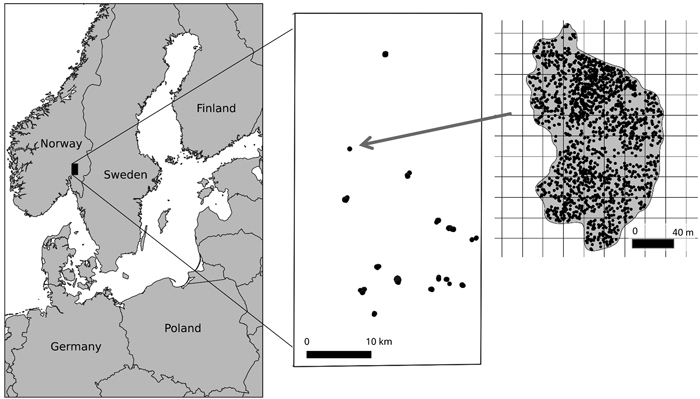
Fig. 1. Location of the study area (left), the distribution of the harvested stands within the study area (middle) and layout of grid cells (harvester plots) within the clear-cut polygon (right). Each harvested stand (middle) or tree (right) is marked with a black dot.
2.1 Harvester data
Harvester data from 47 stands (Fig. 1) were collected in the period January – October 2017 during operational logging with a John Deere 1270E harvester. The harvester was equipped with an integrated positioning system, which enabled accurate positioning of the boom tip of the harvester. This system was used to record and store an accurate position for every individual harvested tree. Two GNSS antennas were mounted at the back of the body of the harvester and seven sensors were mounted on the boom and on the harvester body. It was based on a modified and extended version of the DigPilot positioning system developed by the Norwegian company Gundersen & Løken AS, and is described in more detail by Hauglin et al. (2017, 2018). Control measurements throughout the period of data collection showed a mean positional error of 0.75 m on the single-tree measurements from the harvester (Hauglin et al. 2018).
The information recorded automatically for each tree during the felling operation also included diameter at breast height (DBH), diameter measurements for every 10-cm position along the stem and the length of each log. Using this information, the harvester calculated the volume of all logs and the sum of the log volume was used as an estimate of the merchantable volume of the tree. The harvester operator also recorded manually the tree species and the quality assortment class for each log. All information was recorded and stored in the database in the onboard computer and exported using the StanForD 2010 XML format (Arlinger et al. 2012). The recorded tree positions along with tree sizes and with the three-dimensional point cloud of ALS data for a single stand is illustrated in Fig. 2.
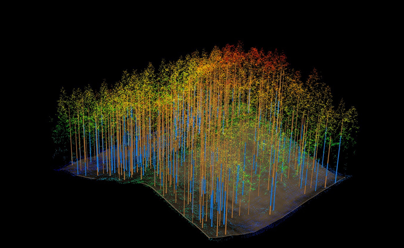
Fig. 2. Example of recorded tree positions along with tree sizes as measured by the harvester and with the three-dimensional point cloud of ALS data for a single stand. The blue and brown colors for the tree stems represent sawn wood and pulpwood, respectively.
The areas covered with harvester data were tessellated into regular grid cells of sizes 200, 400, 900 and 1600 m2 to test different plot sizes. The tessellation process is outlined in the following paragraph. The positioned harvested trees were first used to define polygons of the clear-cut areas. These areas were derived by creating a two-dimensional α-shape from the tree positions using the alphahull package in the R programming software (Pateiro-Lopez and Rodriguez-Casal 2015; R Core Team 2015). A value of 10 m was used for the α parameter. Grids with cell sizes of 200, 400, 900 and 1600 m2 were separately overlaid the harvester data, and grid cells fully within the clear cut polygons were selected for further analysis (Fig. 1). All trees within each of the selected cells were allocated to that cell and used to calculate ground reference data. In the following, we will use the term “harvester plot” to mean one such individual cell. Correspondingly, a stand is defined to be a collection of several spatially contiguous harvester plots. The harvester plots may take the sizes of 200, 400, 900 and 1600 m2 and there are different number of stands associated with the different plot sizes (Table 1).
| Table 1. Mean values (standard deviations in brackets) of the considered attributes at harvester plot and stand level using different harvester plot sizes. | |||||||||
| Plot size (m2) | n | VTotal, m3 ha–1 | VSpruce, m3 ha–1 | VPine, m3 ha–1 | VDeciduous, m3 ha–1 | GTotal, m2 ha–1 | NTotal, ha–1 | VSawSpruce, m3 ha–1 | DmeanSpruce, cm |
| Harvester plot | |||||||||
| 200 | 2306 | 299.0 (138.2) | 260.9 (138.7) | 21.2 (57.5) | 17.0 (38.9) | 27.5 (13.0) | 781 (349.1) | 235.4 (135.6) | 21.9 (4.0) |
| 400 | 949 | 275.1 (115.1) | 242.4 (117.3) | 18.1 (46.9) | 14.7 (30.1) | 25.4 (11.0) | 711 (294.4) | 219.2 (113.7) | 21.9 (3.5) |
| 900 | 285 | 290.8 (90.4) | 258.9 (96.9) | 17.5 (42.9) | 14.5 (27.2) | 27.1 (9.0) | 742.7 (230.3) | 235.0 (94.3) | 21.9 (2.8) |
| 1600 | 99 | 300.0 (66.3) | 272.8 (77.2) | 13.3 (35.5) | 13.9 (21.7) | 28.5 (7.5) | 753.3 (185.9) | 249.3 (75.3) | 22.1 (2.3) |
| Stand | |||||||||
| 200 | 47 | 298.3 (97.7) | 259.3 (103.1) | 17.3 (37.0) | 21.8 (30.8) | 27.6 (8.7) | 808 (222.0) | 232.7 (105.5) | 21.3 (2.8) |
| 400 | 38 | 245.3 (80.8) | 213.6 (84.1) | 19.1 (39.3) | 12.6 (16.1) | 22.6 (7.4) | 660 (211.5) | 190.1 (83.0) | 21.2 (2.9) |
| 900 | 24 | 266.5 (64.9) | 231.4 (67.3) | 24.1 (39.4) | 11.0 (13.1) | 24.6 (6.0) | 733 (148.4) | 203.4 (72.8) | 20.7 (2.6) |
| 1600 | 15 | 281.2 (53.8) | 241.0 (66.1) | 29.8 (48.7) | 10.4 (14.4) | 24.7 (6.4) | 699 (141.5) | 217.1 (63.9) | 21.1 (2.0) |
| VTotal is total merchantable volume and VSpruce, VPine and VDeciduous are merchantable volumes for species Norway spruce, Scots pine and deciduous species, respectively. GTotal and NTotal are basal area and number of stems of the whole living tree stock, respectively. VsawSpruce and DmeanSpruce are merchantable volume of the sawn timber part of the stem diameter distribution and mean diameter of the Norway spruce, respectively. | |||||||||
For each harvester plot size, total number of stems (NTotal) and basal area (GTotal ) were calculated, as well as merchantable volumes by species (VSpruce, VPine, VDeciduous ) and totals (VTotal) (Table 1) . Since Norway spruce is the dominant tree species in the data, additional attributes were calculated for spruce. The stem diameter distribution of spruce was the only one considered. The additional attributes include mean diameter (DmeanSpruce), merchantable volume of the sawn timber part of the stem diameter distribution (VsawSpruce) and cumulative diameter percentiles of 5%, 20%, 30%, 40%, 50%, 60%, 70%, 80% and 95% (D05, …, D95) of the total number of trees in each plot. These percentiles describe the different parts of the distribution. All considered attributes were based on the stem diameter distribution and can be calculated using tree diameters. Corresponding calculations were also made at stand level which consisted of all harvester plots within the respective stands. These calculations were repeated for each plot size (Table 1). In validation only parts of the data were used and mean values of these data sets are shown in Supplementary files S1 and S2.
2.2 ALS data
ALS data were acquired during July 2013 using a fixed-wing aircraft carrying a Leica ALS70 instrument. The pulse repetition frequency was 104.6 kHz and the average flying altitude was 3000 m above ground. The resulting average point density on the ground was 0.7 points m–2. The Terrascan software (Soininen 2016) was used to classify the echoes into ground and above-ground echoes following the methodology described by Axelsson (1999). The above-ground height for all non-ground echoes was calculated as the vertical distance from a triangulated irregular network created from the ground echoes.
The ALS instrument was able to record multiple echoes for each pulse and two datasets were extracted, i.e., 1) a set of first return echoes and 2) a set of last return echoes. Echoes from pulses with only a single echo were included in both datasets. Based on echoes from these two ALS datasets numerical metrics were calculated for each harvester plot. The calculated metrics are described in Table 2.
| Table 2. Description of the metrics derived from the height distribution of the ALS data for individual harvester plots. The metrics were calculated separately for the two respective sets of first return and last return echoes. All metrics where calculated using only the canopy echoes (height > 2 m), with the exception of the density metrics where the total number of echoes also included echoes with height < 2 m. | |
| Metric | Description |
| Hmean | Mean canopy echo height. |
| Hsd | Standard deviation of the canopy echo height distribution. |
| Hcv | Coefficient of variance for the canopy echo height distribution. |
| Hkurt | Kurtosis of the canopy echo height distribution. |
| Hskewness | Skewness of the canopy echo height distribution. |
| H10,, ..., H90 | The 10th, 20th, ..., 90th percentile of the of the canopy echo heights. |
| d0, d1, …, d10 | Density metrics: The height range between the lowest canopy echo and the 95% percentile was divided into 10 fractions of equal length and metrics were computed as the number of echoes above each fraction divided by the total number of echoes (including echoes with height < 2 m). |
2.3 Predicting plot level stem diameter distribution and related attributes using ALS data
The stem diameter distributions were predicted separately using harvester plots of sizes 200, 400, 900 and 1600 m2. The modelling of the stem diameter distributions was carried out by applying a non-parametric approach. Tree lists were predicted using the nearest neighbor (k-nn) imputation and canonical correlation analysis to produce a weighting matrix to select the training harvester plots which were most similar to the target harvester plot in terms of the predictor variables. The k-nn method follows the description by Moeur and Stage (1995), except that the predictions were calculated as weighted averages of the k nearest observations employing weights (W) from the inverse of the canonical correlation analysis-based distance. This approach was chosen according to earlier experiences of multivariate prediction (Packalén and Maltamo 2008; Breidenbach et al. 2010; Maltamo et al. 2018). In the current study, the dependent variables in the canonical correlation analysis were the merchantable volumes by tree species, merchantable volume of saw-log sized trees of spruce and diameters of the 5th, 30th, 50th, 70th and 95th percentiles of the stem diameter distribution of spruce. The value of k was set to 5 based on iterations varying k from 1 to 10 to minimize the error of the predicted diameter percentiles. The number of ALS metrics used in the iterative variable selection (Gill et al. 1981) was 15. This k-nn configuration was used for all harvester plot sizes. The k-nn was implemented using the yaImpute package in R (Crookston and Finley 2008).
As a result of the k-nn analysis the predicted stem diameter distributions consisted of trees observed in the chosen training harvester plots. When constructing a stem diameter distribution for the target harvester plot, the stem frequency represented by each tree of the training harvester plots is required. The harvester plot level weight Wuj of the training harvester plot u and the target harvester plot j was used for this purpose. The harvester plot level weights of k neighbours sum to one.
Let Tuj denote a set of trees t that are predicted from the training harvester plot u for the target harvester plot j, and let n denote the number of trees in u:
![]()
Then the eventual set of trees predicted from the k nearest training harvester plots for the target harvester plot is:
![]()
(Packalén and Maltamo 2008).
From the imputed tree lists all stand attribute predictions of interest were calculated. Those include merchantable volume, basal area and number of stems for the total tree stock calculated from tree list predictions of total stock. Additionally, species-specific merchantable volumes were calculated according to species-specific tree lists. For spruce, also mean diameter, merchantable volume of the sawn timber part of the stem diameter distribution and diameter percentiles at 20%, 40%, 60% and 80% (those percentiles that were not used as dependent variables in the canonical correlation analysis) were predicted. All the above mentioned attributes were validated at stand level.
2.4 Model assessment and estimation accuracy
Accuracy assessment was carried out through a cross validation procedure in which all harvester plots within a stand were excluded from the training data when predicting for harvester plots of this particular stand (leave-one-stand-out cross validation). Hauglin et al. (2018) presented a variogram showing that the merchantable volumes were spatially correlated within a range of about 200 m in the current dataset. Therefore, we also excluded all harvester plots of neighboring stands for which the distance was smaller than 200 m to the particular stand subject to estimation in the cross validation routine. Thus, 0–4 neigboring stands were excluded in the cross validation. The estimates at stand level were obtained as the mean values over all harvester plots within a stand.
Stand-level comparison was carried out in two ways. First, only stands larger than 0.5 hectares were taken into account. This was done in order to get an area corresponding to the typical size of a forest stand. There were also smaller stands that were either originally small (<0.5 ha) or contained only a couple or just a single harvester plot due to the irregular shape. It is worth noting that there are then 19, 18, 4 and 8 stands for the harvester plot sizes 200, 400, 900 and 1600 m2, respectively. Caution should therefore be exercised when comparing the reported results across stand sizes to 1600 m2. Second, all stands large enough to contain harvester plots of 1600 m2 were compared. This comparison was based on 15 stands and included also stands smaller than 0.5 ha. This was done to compare the effect of harvester plot size for the very same stands across all plot sizes. The mean characteristics of both validation cases are shown in Supplementary files 1 and 2. The accuracy of these estimates was first evaluated in terms of root mean squared error:

where n is the number of stands, ![]() is the observed value for stand i, and
is the observed value for stand i, and ![]() is the estimated value for stand i.
is the estimated value for stand i. Subsequently, the RMSE% was calculated by dividing the RMSE by the estimated mean of the attribute in question.
Secondly, a validation was performed for the stem diameter distribution (1-cm classes) of Norway spruce by applying the variant of error index by Reynolds et al. (1988) presented by Packalén and Maltamo (2008) which is determined as follows:

where fi and ![]() refer to the number of observed and estimated trees in the classes of the stem diameter distribution, l is the number of classes in the stem diameter distribution, and N and
refer to the number of observed and estimated trees in the classes of the stem diameter distribution, l is the number of classes in the stem diameter distribution, and N and ![]() represent the number of observations in the observed and estimated distributions, respectively. Also here stand-level observed stem diameter distributions and stand-level averaged estimated tree lists were compared.
represent the number of observations in the observed and estimated distributions, respectively. Also here stand-level observed stem diameter distributions and stand-level averaged estimated tree lists were compared.
3 Results
The results of the validation of the k-nn predictions of the different stand attributes at stand level for stands larger than 0.5 hectares using different harvester plot sizes are shown in Table 3. The estimation errors of total merchantable volume were smaller than 10% for the 200 m2 and 400 m2 harvester plot sizes, whereas for merchantable volume of spruce the errors were smaller than 20% with the exception of the harvester plot size of 900 m2. The errors were a little bit larger for the saw-log part of the distribution. The RMSE of the most accurate total merchantable volume prediction was about 25 m3 ha–1. For minor tree species, the errors were considerably larger and they differed between harvester plot sizes. Scatterplots showing merchantable volume estimations for different plot sizes are displayed in Fig. 3. These scatterplots show linear relationships, except in the case of 1600 m2 where the estimations are considerably averaged and four of these estimates are almost on a horizontal line.
| Table 3. Estimation errors indicated by RMSE% (RMSE values in brackets) of different total and species-specific stand attributes with different harvester plot sizes. | ||||
| Plot size 200 m2 | Plot size 400 m2 | Plot size 900 m2 | Plot size 1600 m2 | |
| Number of stands | 19 | 18 | 14 | 8 |
| VTotal , m3 ha–1 | 8.4 (25.5) | 9.5 (26.0) | 11.6 (32.9) | 11.9 (35.2) |
| NTotal, ha–1 | 19.3 (144.9) | 17.8 (123.0) | 16.3 (116.2) | 14.3 (104.6) |
| GTotal, m2 ha–1 | 9.1 (2.9) | 9.8 (2.8) | 12.5 (3.7) | 13.0 (4.0) |
| VSpruce, m3 ha–1 | 18.9 (47.7) | 18.96 (46.0) | 22.5 (57.6) | 19.1 (52.2) |
| VPine, m3 ha–1 | 140.1 (33.5) | 169.2 (33.1) | 237.4 (41.1) | 193.1 (21.8) |
| VDeciduous, m3 ha–1 | 85.4 (12.4) | 96.7 (12.5) | 140.8 (15.1) | 136.4 (16.9) |
| VsawSpruce, m3 ha–1 | 20.3 (49.0) | 22.0 (48.5) | 26.2 (61.1) | 22.3 (55.9) |
| DmeanSpruce, cm | 10.6 (2.3) | 11.0 (2.4) | 12.0 (2.6) | 9.7 (2.2) |
| D20, cm | 14.0 (2.0) | 15.2 (2.2) | 18.3 (2.7) | 16.8 (2.5) |
| D40, cm | 12.7 (2.4) | 13.2 (2.5) | 15.7 (3.0) | 12.8 (2.5) |
| D60, cm | 11.3 (2.6) | 11.5 (2.7) | 12.7 (3.0) | 10.4 (2.5) |
| D80, cm | 10.3 (2.8) | 10.3 (2.9) | 10.0 (2.8) | 8.8 (2.5) |
| Error Index (mean value) | 0.15 | 0.17 | 0.18 | 0.18 |
| D20, D40, D60 and D80 are cumulative diameter percentiles of 20%, 40%, 60% and 80% of the number of stems, respectively. For other abbreviations, see Table 1. | ||||
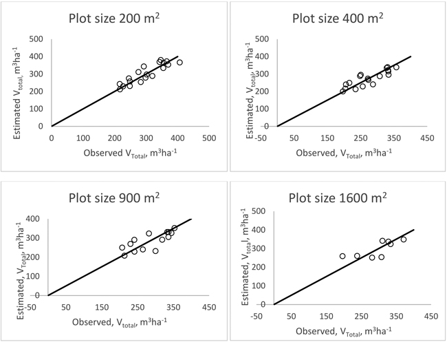
Fig. 3. Merchantable volume estimation validation at stand level using different plot sizes.
The estimation errors of the diameter percentiles were usually smallest for the 50th percentile (i.e. median diameter) and for the largest considered percentile (80th). Most of the percentile figures were fairly accurate showing 10–15% error. The error index values for the different harvester plot sizes were close to each other and smaller than 0.2. Finally, the RMSE values of the number of stems were smaller the larger the plot size and in the case of basal area they were close to corresponding values of merchantable volume.
The results for the same 15 validation stands for all plot sizes are shown in Fig. 4. Also results from the previous validation using stands larger than 0.5 hectares (Table 3) are shown in Fig. 4 for comparison. Only total and spruce merchantable volumes are shown. The results from the analysis of the same stands across all plot sizes were mostly in line with the validation already presented (Table 3). Only in the case of a harvester plot size of 1600 m2 the reliability figures somewhat differed between the two considered validation approaches. For harvester plot sizes 200 and 400 m2 the errors were smaller than 10% and 20% for total merchantable volume and spruce merchantable volume, respectively. For the harvester plot size of 1600 m2 the errors were considerably larger in the analysis based on the same stands across all plot sizes.
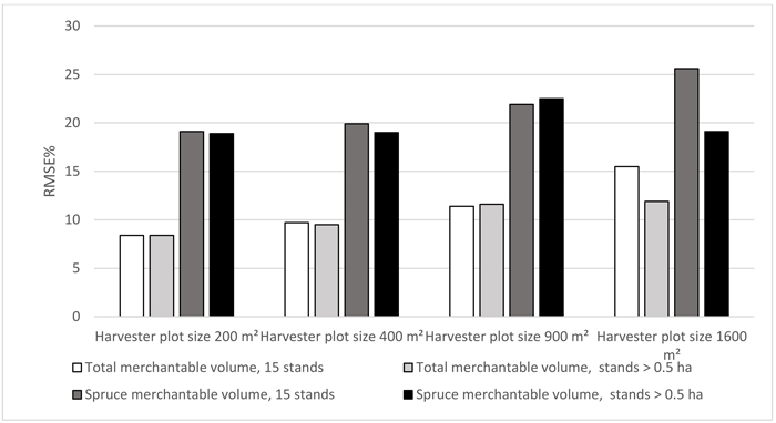
Fig. 4. Estimation errors of total merchantable volume and spruce merchantable volume when the same stands (n = 15) were used in the validation across all harvester plot sizes. Also results from the validation using stands larger than 0.5 hectares are shown for comparison.
Examples of the estimated stand-level spruce stem diameter distributions for a single validation stand are shown in Fig. 5 for different harvester plot sizes using 2 cm classes. The estimated values of the error indices for this stand were 0.14, 0.18, 0.16 and 0.21 for harvester plot sizes of 200, 400, 900 and 1600 m2, respectively. Correspondingly, for those harvester plot sizes, the considered areas of the given stand were 0.7, 0.6, 0.375 and 0.32 hectares. Thus, also the field values of the frequency distributions changed due to the rather small size of the stand. It can be seen from the figures though that the fit was good for all harvester plot sizes. In the case of the smallest harvester plot size (200 m2) the only notable deviations were for diameter classes 18 cm and –20 cm. Among the larger harvester plot sizes, the k-nn based estimates resulted in considerable over-estimation of the frequency of trees in diameter classes 10–14 cm for harvester plot sizes 400 m2 and 900 m2 and in diameter classes 28–38 cm for the harvester plot size of 1600 m2.
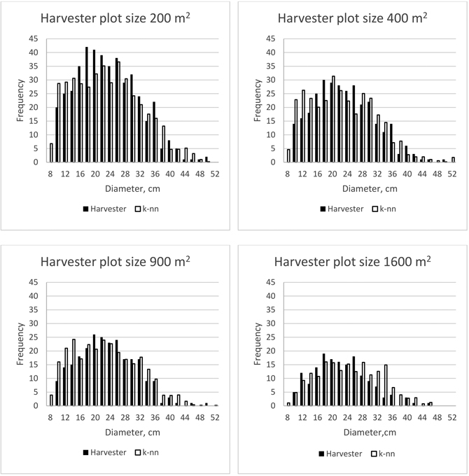
Fig. 5. Example of stand-level stem diameter distributions based on harvester measurements and k-nn based estimation using different harvester plot sizes.
Finally, examples of stem diameter distributions for the plot size 200 m2 of the smallest and largest obtained error index values are shown in Figs. 6 and 7. For the smallest error index value (0.05) the estimate of the stem diameter distribution is very close to the field value (Fig. 6) whereas in the case of the largest error index value (0.22) there is a considerable overestimation, especially in the smaller diameter classes (Fig. 7).
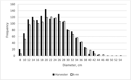
Fig. 6. Stem-level diameter distribution estimate of the smallest error index value (0.05) in the case of plot size 200 m2.
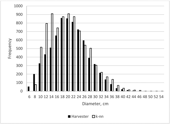
Fig. 7. Stem-level diameter distribution estimate of the largest error index value (0.22) in the case of plot size 200 m2.
4 Discussion
This study examined the use of harvester data in the estimation of stand-level stem diameter distributions and related stand attributes. We also compared different harvester plot sizes in the estimation. Our material consisted of stands formed by aggregating multiple adjacent squared plots. In the stand-level validation, we used the area of all the located harvester plots within a stand. Thus, we were able to perform an evaluation of stand units of considerably larger sizes than in the existing literature. However, there were also stands in the material consisting of just a few harvester plots. All harvester plots were used in the plot level prediction but the validation part of the analysis was carried out by using a lower threshold for inclusion in the analysis of 0.5 hectares. We also compared a sub-set of stands large enough to contain harvester plots of 1600 m2, which allowed comparison for the same stands across all harvester plot sizes. Since this type of field data is collected during a final harvest, only mature stands were included, whereas ALS-based forest inventories typically comprise forests with greater diversity in terms of development stages and stand ages. We also restricted the analysis of volume attributes to merchantable volume, i.e., treetops were excluded, whereas in traditional forest inventories the volume of the entire stem is usually estimated. These aspects must be taken into account when comparing the results of this study to earlier studies reported in the literature.
The stand-level error of merchantable volume was in the most accurate cases smaller than 9% in the current study. This can be considered small and shows the strong relationship between ALS data and ground reference volume. Similar levels of errors have been reported in some previous studies though, like the work by Suvanto et al. (2005) where the validation units in mature forest stands were of size 1000–2000 m2. Furthermore, among a fairly large number of Nordic studies conducted in the period 1995–2010 (Næsset 2014; Maltamo and Packalen 2014), a few have reported stand level volume error of slightly more than 10%, for example Næsset (2007) who used 1000 m2 validation plots in mature stands and Holmgren (2004) who validated the estimates on 0.64 hectare units within stands. The Nordic studies were mainly conducted under boreal forest conditions. Under different growing conditions with more homogeneous stand structures (eucalyptus plantations) Packalén et al. (2011) reported volume errors smaller than 9% using a plot size of approximately 500 m2. When comparing our results to the earlier studies it should be remembered that our study stands are from a small geographical area. However, we excluded neighboring stands closer than 200 m to avoid training data to be used for prediction purposes in the immediate proximity. The 200-m threshold was guided by previous observations of spatial correlation of volume. Some other earlier studies, such as that of Suvanto et al. (2005), were also conducted in rather small geographical area.
One way to analyze our results is to use mean value of field measured stands as a predictor for all stands. In this case the RMSE% values of merchantable volume were 18.4, 21.7, 18.2 and 15.5 for plot sizes 200, 400, 900 and 1600 m2, respectively. Here the difference between k-nn prediction and mean value-based prediction shows the improvement due to the use of the ALS data. For example, in the case of 200 and 400 m2 plot sizes the improvement is about ten percentage units but only negligible for the 1600 m2 plot size showing the averaging effect of larger plot size.
The accuracy levels of the current study are comparable to earlier results but not exceptionally better, even though the area of the validation units was considerably larger. Usually prediction errors decrease when averaging the predictions over a larger area. However, under typical boreal forest conditions there seems to be an asymptotic tendency of the averaging effect on the accuracy around, say, 1000–2000 m2. That was also the justification for exploring and choosing validation plot sizes of around 1000–4000 m2 in the early Nordic studies (Næsset 2002, 2004a, b). It should be remembered though, that here we consider merchantable volume and there are additional error sources in the presented approach to use harvester data, such as for example various types of mismatch between the ALS data and harvester data. As mentioned by Hauglin et al. (2018), the retention trees that are measured during an ALS campaign and consequently are reflected in the ALS metrics but which are not cut by harvester, will have an effect on the accuracy of volume predictions. Secondly, errors in tree positions will cause a mismatch between ALS and harvester data. A harvested tree may be assigned to different harvester plots in the harvester data than in the ALS data. This positional error can typically be up to around 2 m (Hauglin et al. 2017). In the current data, there was also a time lag of 4 yrs between the harvester data and the ALS data.
The possible mismatch between ALS data and harvester plots is also evident in the harvester plot-level errors of the k-nn predictions. In this study, we have only reported stand-level validation results. However, for the harvester plot sizes of 200, 400, 900 and 1600 m2, the obtained RMSE% values for merchantable volume were 33.3, 31.9, 22.9, and 18.9, respectively. In the case of harvester plot sizes of 200 and 400 m2 these values are rather large when compared to typical values of ALS-based forest inventory, but nevertheless comparable to the results for harvester data reported by Hauglin et al. (2018). It is worth noting that for the largest harvester plot sizes the improvement in RMSE% from harvester plot to stand level was rather small. If different harvester plot sizes are compared to each other it can be seen that at harvester plot level the accuracy was highest for the largest harvester plot size. However, also the variability of the considered attributes were smaller for larger harvester plot sizes (Table 1). At stand level the situation was opposite; the largest harvester plot size had usually the largest RMSE% values. In the case of the 1600 m2 plot size the small size of the training data may have affected the stand level cross validation for some stands. For example, Maltamo et al. (2009a) showed that the accuracy of k-nn based predictions of stem diameter distribution decreased when the number of observations in the training dataset was less than 100. There were some exceptions though, such as for estimates of number of stems and mean diameter where the accuracy of the largest harvester plot size at stand level was comparable to the other plot sizes. It must be remembered that when tessellating the stands into differently sized harvester plots the covered area will differ and those stands used in the assessment will also partly differ between plot sizes. We wanted to avoid the latter effect and, therefore, also conducted an alternative analysis comparing only those stands that were present across all plot sizes. The effect of harvester plot size was however more or less the same in both analyses. For smaller harvester plot sizes, i.e., 200, 400 and 900 m2, the stand-level differences between accuracies were usually smaller.
The applied nearest neighbor approach imputed tree lists of all species simultaneously and stand totals were estimated as a sum of them. We were primarily interested in stem diameter distribution of Norway spruce for mature stands since this species is the dominant one and also the economically most important in the study area. Even though our suite of predictor variables did not include for example spectral information or leaf-off or multispectral ALS data which have been found useful to separate species (Packalén and Maltamo 2007; Villikka et al. 2012; Budei et al. 2018), the accuracy for spruce seemed to be very good at stand level. Also here we conducted an analysis with mean value of field measured stands as a predictor for all stands. In this case the RMSE% values of merchantable spruce volume were 18.8, 22.7, 20.6 and 20.5 for plot sizes 200, 400, 900 and 1600 m2, respectively. These results show that the effect of ALS data-based species specific prediction is negligible. Thus, the good accuracy level is due to both the averaging effect for larger areas and especially the great dominance of spruce in the study area.
When considering different attributes related to stem diameter distribution it can be seen that, for example, the error levels of the diameter percentile predictions were rather low. Correspondingly, the average error index values were less than 0.2, a level which is much lower than obtained in validations in earlier studies. For example, Packalén and Maltamo (2008) obtained error index values between 0.2 and 0.3 while Maltamo et al. (2009a) obtained values >0.3. In addition, the visual inspection of the estimated distributions showed a high level of similarity (Figs. 5–7). The averaging effect from plot to stand can be seen also here. When using for example the harvester plot size of 200 m2 the error index at harvester plot level was 0.66 and at stand level 0.15. This further indicates a close relationship between ALS-based stem diameter distribution estimates and field measurements at stand level. The stand-level attributes estimated from the stem diameter distributions for Norway spruce also showed smaller errors for harvester plot sizes of 200 and 400 m2 than for larger harvester plot sizes. Another benefit of smaller harvester plot sizes is the possibility to locate the harvester plots in smaller stands and thereby obtain a larger number of training data observations as well as having more stands represented in the sample.
In our case we wanted to use all the information available for different harvester plot sizes and, therefore, compared partly different stands and stand areas. Another possibility would have been to examine the effect of harvester plot sizes using exactly the same areas within a stand and even the same number of training harvester plots for k-nn analysis. This could be a subject for future investigations.
The approach of utilizing tree-level positioned harvester data in construction of harvester plots showed good performance in estimating attributes that may be computed from a stem diameter distribution. Peuhkurinen et al. (2008) used harvester data for imputing saw-log recoveries. The k-nn analysis was performed at stand level and, thus, the training data were restricted to a rather small sample size; 35 stands in total. In contrast, the tree-level positioning that we adopted in the current study, offered as many as 2306 harvester plots in 47 stands as training data when a plot size of 200 m2 was chosen. The choice of a harvester plot size for a given application is also flexible when tree-level positioning is applied. Tree-level positioned harvester data can be utilized in many different contexts. Maybe one of the most obvious ones is in pre-harvest inventory for a given mature stand where an existing stem data bank of the same dominating tree species is used as training data. Results of this study show that the accuracy of the estimated stem diameter distribution may be appropriate for planning of the bucking.
5 Conclusions
We studied the estimation of stand-level stem diameter distribution and related attributes using tree-level positioned harvester plots and ALS data. The results show a close relationship between ALS and harvester data, indicating the suitability of harvester data to estimate stand attributes of mature spruce-dominated stands. The approach can be utilized especially in a pre-harvest inventory context. We also compared different harvester plot sizes and conclude that smaller plot size, say, 200–400 m2 is optimal for stand level estimation when applying plot level non-parametric prediction. Thus, the current practice of adopting a plot radius between 8 and 12 m seems to be appropriate. The utilization of tree-level positioned harvester data is a flexible approach to use those plot sizes that are optimal for any particular application.
Acknowledgements
We would like to thank Gundersen & Løken AS, John Deere Forestry Norway AS, Viken Skog SA, and Røsåsen Skogsmaskiner AS for cooperation on the development, implementation, and evaluation of the positioning system. We would further like to thank Steinar Sætha and Steinar Åmål at Røsåsen Skogsmaskiner AS for operating the harvester and M.Sc. Janne Räty for technical support. The study was funded by the Research Council of Norway as part of the projects entitled “Sustainable Utilization of Forest Resources in Norway” (grant 225329/E40) and “Precision forestry for improved resource utilization and reduced wood decay in Norwegian forests (PRECISION)” (grant 281140) and the Academy of Finland; FORBIO (The Strategic Research Council, Grant No. 314224).
References
Arlinger J., Nordström M., Möller J.J. (2012). StanForD 2010: modern kommunikation med skogsmaskiner. Skogforsk. 16 p.
Axelsson P.E. (1999). Processing of laser scanner data—algorithms and applications. ISPRS Journal of Photogrammetry and Remote Sensing 54(2–3): 138–147. https://doi.org/10.1016/S0924-2716(99)00008-8.
Barth A., Holmgren J. (2013). Stem taper estimates based on airborne laser scanning and cut-to-length harvester measurements for pre-harvest planning. International Journal of Forest Engineering 24(3): 161–169. https://doi.org/10.1080/14942119.2013.858911.
Bollandsås O.M., Maltamo M., Gobakken T., Næsset E., Lien V. (2011). Prediction of timber quality parameters of forest stands by means of small footprint airborne laser scanner data. International Journal of Forest Engineering 22(1): 14–23. https://doi.org/10.1080/14942119.2011.10702600.
Breidenbach J., Næsset E., Lien V., Gobakken T., Solberg S. (2010). Prediction of species-specific forest inventory attributes using a nonparametric semi-individual tree crown approach based on fused airborne laser scanning and multispectral data. Remote Sensing of Environment 114(4): 911–924. https://doi.org/10.1016/j.rse.2009.12.004.
Budei B.C., St-Onge B., Hopkinson C., Audet F.-A. (2018). Identifying the genus or species of individual trees using a three-wavelength airborne lidar system. Remote Sensing of Environment 204: 632–647. https://doi.org/10.1016/j.rse.2017.09.037.
Crookston N.L., Finley A.O. (2008). yaImpute: an R package for kNN imputation. Journal of Statistical Software 23(10): 1–16. https://doi.org/10.18637/jss.v023.i10.
Gill P.E., Murray W., Wright M. (1981). Practical Optimization. Academic Press Inc, London. 401 p.
Gobakken T., Næsset E. (2004). Estimation of diameter and basal area distributions in coniferous forest by means of airborne laser scanner data. Scandinavian Journal of Forest Research 19(6): 529–542. https://doi.org/10.1080/02827580410019454.
Gobakken T., Næsset E. (2008). Assessing effects of laser point density, ground sampling intensity, and field sample plot size on biophysical stand properties derived from airborne laser scanner data. Canadian Journal of Forest Research 38(5):1095–1109. https://doi.org/10.1139/X07-219.
Hauglin M., Hansen E., Næsset E., Busterud B.E., Omholt Gjevestad J.G., Gobakken T. (2017). Accurate Single-Tree Positions from a Harvester: A Test of Two Global Satellite-Based Positioning Systems. Scandinavian Journal of Forest Research 32(8): 774–781. https://doi.org/10.1080/02827581.2017.1296967.
Hauglin M., Hansen E., Sørngård E., Næsset E., Gobakken T. (2018). Utilizing accurately positioned harvester data: Modelling forest volume with airborne laser scanning. Canadian Journal of Forest Research 48(8): 913–922. https://doi.org/10.1139/cjfr-2017-0467.
Hawbaker T.J., Keuler N.S., Lesak A.A., Gobakken T., Contrucci K., Radeloff V.C. (2009). Improved estimates of forest vegetation structure and biomass with a LiDAR-optimized sampling design. Journal of Geophysical Research 114(G2): G00E04. https://doi.org/10.1029/2008JG000870.
Holmgren J. (2004). Prediction of tree height, basal area and stem volume in forest stands using airborne laser scanning. Scandinavian Journal of Forest Research 19(6): 543–553. https://doi.org/10.1080/02827580410019472.
Holmgren J., Barth A., Larsson H., Olsson H. (2012). Prediction of stem attributes by combining airborne laser scanning and measurements from harvesters. Silva Fennica 46(2): 227–239. https://doi.org/10.14214/sf.56.
Koivuniemi J., Korhonen K.T. (2006). Inventory by compartments. In: Kangas A., Maltamo M. (eds.). Forest inventory. Methodology and applications. Managing Forest Ecosystems, vol 10. Springer, Dordrecht. p. 271–278. https://doi.org/10.1007/1-4020-4381-3_16.
Kotivuori E. Maltamo M., Korhonen L., Packalen P. (2018). Calibration of nationwide airborne laser scanning based stem volume models. Remote Sensing of Environment 210: 179–192. https://doi.org/10.1016/j.rse.2018.02.069.
Lindroos O., Ringdahl O., La Hera P., Hohnloser P., Hellstrom T. (2015). Estimating the position of the harvester head – a key step towards the Precision Forestry of the future? Croatian Journal of Forest Engineering 36: 147–164.
Malinen J., Maltamo M., Harstela P. (2001). Application of most similar neighbor inference for estimating characteristics of a marked stand characteristics using harvester and inventory generated stem databases. International Journal of Forest Engineering 12(2): 33–41. https://doi.org/10.1080/14942119.2001.10702444.
Maltamo M., Næsset E., Bollandsås O.-M., Gobakken T., Packalén P. (2009a). Non-parametric estimation of diameter distributions by using ALS data. Scandinavian Journal of Forest Research 24(6): 541–553. https://doi.org/10.1080/02827580903362497.
Maltamo M., Packalén P., Suvanto A., Korhonen K.T., Mehtätalo L., Hyvönen P. (2009b). Combining ALS and NFI training data for forest management planning: a case study in Kuortane, Western Finland. European Journal of Forest Research 128(3): 305–317. https://doi.org/10.1007/s10342-009-0266-6.
Maltamo M., Packalen P. (2014). Species specific management inventory in Finland. In Forestry Applications of Airborne Laser Scanning –concepts and case studies. M. Maltamo E. Næsset and J. Vauhkonen (eds.). Managing Forest Ecosystems, vol. 27. Springer, Dordrecht. p. 241–252. https://doi.org/10.1007/978-94-017-8663-8_12.
Maltamo M., Mehtätalo L., Valbuéna R., Vauhkonen J., Packalen P. (2018). Airborne laser scanning for tree diameter distribution modelling: a comparison of different modeling alternatives in a tropical single-species plantation. Forestry 91(1): 121–131. https://doi.org/10.1093/forestry/cpx041.
Moeur M., Stage A.R. (1995). Most similar neighbor: an improved sampling inference procedure for natural resource planning. Forest Science 41: 337–359.
Næsset E. (2002). Predicting forest stand characteristics with airborne scanning laser using a practical two-stage procedure and field data. Remote Sensing of Environment 80(1): 88–99. https://doi.org/10.1016/S0034-4257(01)00290-5.
Næsset E. (2004a). Practical large-scale forest stand inventory using small-footprint airborne scanning laser. Scandinavian Journal of Forest Research 19(2): 164–179. https://doi.org/10.1080/02827580310019257.
Næsset E. (2004b). Accuracy of forest inventory using airborne laser-scanning: evaluating the first Nordic full-scale operational project. Scandinavian Journal of Forest Research 19(6): 554–557. https://doi.org/10.1080/02827580410019544.
Næsset E. (2007). Airborne laser scanning as a method in operational forest inventory: status of accuracy assessments accomplished in Scandinavia. Scandinavian Journal of Forest Research 22(5): 433–442. https://doi.org/10.1080/02827580701672147.
Næsset E., Gobakken T., Solberg S., Gregoire T.G., Nelson R., Ståhl G., Weydahl D. (2011). Model assisted regional forest biomass estimation using LiDAR and InSAR as auxiliary data: a case study from a boreal forest area. Remote Sensing of Environment 115(12): 3599–3614. https://doi.org/10.1016/j.rse.2011.08.021.
Næsset E. (2014) Area-based inventory in Norway – from innovation to an operational reality. In: Maltamo M., Næsset E., Vauhkonen J. (eds.). Forestry applications of airborne laser scanning – concepts and case studies. Managing Forest Ecosystems, vol 27. Springer, Dordrecht. p. 215–240. https://doi.org/10.1007/978-94-017-8663-8_11.
Nilsson M., Nordkvist K., Jonzéna J., Lindgren N., Axenstena P., Wallerman J., Egberth M., Larsson S., Nilsson L., Eriksson J., Olsson H. (2017). A nationwide forest attribute map of Sweden predicted using airborne laser scanning data and field data from the National Forest Inventory. Remote Sensing of Environment 194: 447–454. https://doi.org/10.1016/j.rse.2016.10.022.
Olivera A., Visser R. (2016). Development of forest-yield maps generated from Global Navigation Satellite System (GNSS)-enabled harvester StanForD files: preliminary concepts. New Zealand Journal of Forestry Science 46:3.
Packalén P., Maltamo M. (2007). The k-MSN method in the prediction of species specific stand attributes using airborne laser scanning and aerial photographs. Remote Sensing of Environment 109(3): 328–341. https://doi.org/10.1016/j.rse.2007.01.005.
Packalén P., Maltamo M. (2008). The estimation of species-specific diameter distributions using airborne laser scanning and aerial photographs. Canadian Journal of Forest Research 38(7): 1750–1760. https://doi.org/10.1139/X08-037.
Packalén P., Mehtätalo L., Maltamo M. (2011). ALS based estimation of plot volume and site index in a Eucalyptus plantation with a nonlinear mixed effect model that accounts for the clone effect. Annals of Forest Science 68: 1085–1092. https://doi.org/10.1007/s13595-011-0124-9.
Pateiro-Lopez B., Rodriguez-Casal A. (2015). R package alphahull: generalization of the convex hull of a sample of points in the plane. https://CRAN.R-project.org/package=alphahull.
Peuhkurinen J., Maltamo M., Malinen J. (2008). Estimating species-specific height-diameter distributions and saw log recoveries from ALS data and aerial photographs: a distribution-based approach. Silva Fennica 42(4): 625–641. https://doi.org/10.14214/sf.237.
R Core Team. (2015). R: a language and environment for statistical computing. R Foundation for Statistical Computing, Vienna, Austria. https://www.R-project.org/.
Rasinmäki J., Melkas T. (2005). A method for estimating tree composition and volume using harvester data. Scandinavian Journal of Forest Research 20(1): 85–95. https://doi.org/10.1080/02827580510008185.
Reynolds M.R. Jr., Burk T.E., Huang W.-C. (1988). Goodness-of-fit tests and model selection procedures for diameter distribution models. Forest Science 34: 373–399.
Shang C., Treitz P., Caspersen J., Jones T. (2017). Estimating stem diameter distributions in a management context for a tolerant hardwood forest using ALS height and intensity data. Canadian Journal of Remote Sensing 43(1): 79–94. https://doi.org/10.1080/07038992.2017.1263152.
Siipilehto J., Lindeman H., Vastaranta M., Xiaowei Y., Uusitalo J. (2016). Reliability of the predicted stand structure for clearcut stands using optional methods: airborne laser scanning-based methods, smartphone-based forest inventory application Trestima and pre-harvest measurement tool EMO. Silva Fennica 50(3) article 1568. https://doi.org/10.14214/sf.1568.
Soininen A. (2016). TerraScan user’s guide. Jyväskylä, Finland. Terrasolid Oy.
Ståhl G., Holm S., Gregoire T., Gobakken T., Næsset E., Nelson R. (2011). Model-based inference for biomass estimation in a LiDAR sample survey in Hedmark County, Norway. Canadian Journal of Forest Research 41(1): 96–107. https://doi.org/10.1139/X10-161.
Suvanto A., Maltamo M., Packalén P., Kangas J. (2005). Kuviokohtaisten puustotunnusten ennustaminen laserkeilauksella. Metsätieteen aikakauskirja 4/2005: 413–428. [In Finnish]. https://doi.org/10.14214/ma.6138.
Tuominen S., Pitkänen J., Balazs A., Korhonen K.T., Hyvönen P., Muinonen E. (2014). NFI plots as complementary reference data in forest inventory based on airborne laser scanning and aerial photography in Finland. Silva Fennica 48(2) article 983. https://doi.org/10.14214/sf.983.
Villikka M., Packalén P., Maltamo M. (2012). The suitability of leaf-off airborne laser scanner data for forest inventory. Silva Fennica 46(1): 99–110. https://doi.org/10.14214/sf.68.
White J.C., Wulder M.A., Varhola A., Vastaranta M., Coops N.C., Cook B.D., Pitt D., Woods M. (2013). A best practices guide for generating forest inventory attributes from airborne laser scanning data using an area-based approach. Forest Chronicle 89(6): 722–723. https://doi.org/10.5558/tfc2013-132.
Total of 48 references.
