Lennart Noordermeer  ,
Hans Ole Ørka,
Terje Gobakken
,
Hans Ole Ørka,
Terje Gobakken
Imputing stem frequency distributions using harvester and airborne laser scanner data: a comparison of inventory approaches
Noordermeer L., Ørka H. O., Gobakken T. (2023). Imputing stem frequency distributions using harvester and airborne laser scanner data: a comparison of inventory approaches. Silva Fennica vol. 57 no. 3 article id 23023. https://doi.org/10.14214/sf.23023
Highlights
- We imputed stem frequency distributions using harvester reference data and predictor variables computed from airborne laser scanner data.
- Stand-level distributions of stem diameter, tree height, volume, and sawn wood volume
- (Enhanced) area-based and semi-individual tree crown approaches outperformed the individual tree crown method.
Abstract
Stem frequency distributions provide useful information for pre-harvest planning. We compared four inventory approaches for imputing stem frequency distributions using harvester data as reference data and predictor variables computed from airborne laser scanner (ALS) data. We imputed distributions and stand mean values of stem diameter, tree height, volume, and sawn wood volume using the k-nearest neighbor technique. We compared the inventory approaches: (1) individual tree crown (ITC), semi-ITC, area-based (ABA) and enhanced ABA (EABA). We assessed the accuracies of imputed distributions using a variant of the Reynold’s error index, obtaining the best mean accuracies of 0.13, 0.13, 0.10 and 0.10 for distributions of stem diameter, tree height, volume and sawn wood volume, respectively. Accuracies obtained using the semi-ITC, ABA and EABA inventory approaches were significantly better than accuracies obtained using the ITC approach. The forest attribute, inventory approach, stand size and the laser pulse density had significant effects on the accuracies of imputed frequency distributions, however the ALS delay and percentage of deciduous trees did not. This study highlights the utility of harvester and ALS data for imputing stem frequency distributions in pre-harvest inventories.
Keywords
forest inventory;
airborne laser scanning;
harvester data;
inventory approaches
-
Noordermeer,
Faculty of Environmental Sciences and Natural Resource Management, Norwegian University of Life Sciences, P.O. Box 5003, NO-1432 Ås, Norway
 https://orcid.org/0000-0002-8840-0345
E-mail
lennart.noordermeer@nmbu.no
https://orcid.org/0000-0002-8840-0345
E-mail
lennart.noordermeer@nmbu.no
-
Ørka,
Faculty of Environmental Sciences and Natural Resource Management, Norwegian University of Life Sciences, P.O. Box 5003, NO-1432 Ås, Norway
https://orcid.org/0000-0002-7492-8608
E-mail
hans-ole.orka@nmbu.no
- Gobakken, Faculty of Environmental Sciences and Natural Resource Management, Norwegian University of Life Sciences, P.O. Box 5003, NO-1432 Ås, Norway E-mail terje.gobakken@nmbu.no
Received 24 April 2023 Accepted 2 October 2023 Published 9 October 2023
Views 66649
Available at https://doi.org/10.14214/sf.23023 | Download PDF

1 Introduction
Accurate and high-resolution information on forest attributes is essential for optimizing forest management and wood procurement (Duvemo and Lämås 2006). In the Nordic countries, forest stands are the primary unit in forest planning. Decision support systems used in forest planning rely on information on forest resources, commonly in the form of stand averages and totals, such as basal area, tree height and numbers of stems (Eid and Hobbelstad 2000). Besides averages and totals, stem frequency distributions, such as diameter distributions, have been a key source of information both in long-term forest planning (Saad et al. 2015) and tactical, pre-harvest planning (Peuhkurinen et al. 2007). Distributions provide information on potential timber assortments, the forest structure, and the silvicultural state of a stand (Uuttera and Maltamo 1995; Kuuluvainen et al. 1996). In addition, information on individual trees can be derived from the distributions, which allow for simulating future stand development (Wikström et al. 2011).
Airborne laser scanning (ALS) has been a main data source for forest inventory over the past decades (Maltamo et al. 2014). ALS data provide spatially continuous and detailed information on forest structure as well as terrain height and allow for estimating a range of forest attributes. Two main inventory approaches are commonly used in estimating forest attributes from ALS data. The area-based approach (ABA; Næsset 2002) is used most frequently, by which ALS metrics are calculated for sample plots and linked to the plots’ forest attributes in statistical models. The models are then used to predict the corresponding attributes over a grid tessellating the inventory area. Alternatively, the individual tree crown (ITC) approach has been proposed to provide tree-level information for tree crown segments delineated from ALS data (Brandtberg 1999; Hyyppä 1999). In the ITC approach, tree crowns of individual trees are segmented from ALS data and tree attributes are then predicted from the ALS data for each segment (Dalponte et al. 2018).
The ABA approach is practical in terms of field work, as co-location between field plot data and ALS data is conveniently done using coordinates of sample plot centers. However, the ABA can in some cases be susceptible to edge effects along borders of sample plots and grid cells, potentially leading to systematic errors (Næsset et al. 2013; Packalén et al. 2015). The ITC approach, on the other hand, relies on the capabilities of algorithms to derive the positions and heights of detected trees from the ALS data (Pascual 2019). Resultingly, only 30–70% of trees can be expected to be delineated (Kaartinen et al. 2012; Vauhkonen et al. 2012), whereby larger trees are more likely to be detected (Solberg et al. 2006). Further, tree crown segments are assumed to contain only a single tree, which can result in additional systematic errors in estimates of forest attributes (Persson et al. 2002; Peuhkurinen et al. 2011).
Variations on the ABA and ITC approaches have emerged to mitigate the mentioned sources of error. Packalén et al. (2015) proposed the enhanced ABA (EABA), in which edge effects due to tree crowns overlapping boundaries of sample plots and grid cells are accounted for. In the approach, boundaries of plots and cells are adjusted for tree crowns segmented from the ALS data, whereby crown segments of “in” trees are merged with the cell, and crown segments of “out” trees are discarded from the cell. This has been shown to resolve edge effects as well as co-registration between reference data and ALS data (Pascual 2019). Breidenbach et al. (2010) proposed the semi-ITC approach to account for systematic errors resulting from trees missing in the ITC data. In the semi-ITC approach, tree crown segments can contain single, multiple or no trees, which can reduce systematic errors substantially as shown by Kandare et al. (2017).
Besides being a useful data source for prediction of forest attributes at tree- and plot-level, ALS data have proven useful for estimating stem frequency distributions, mainly diameter distributions (Gobakken and Næsset 2004; Maltamo et al. 2006). However, few studies have assessed the use of ALS data for prediction of distributions of attributes other than stem diameter. Peuhkurinen et al. (2008) predicted height-diameter distributions at stand level to subsequently predict saw log recoveries from a stem bank. Mehtätalo et al. (2015) demonstrated a method for predicting tree height distributions from ALS data at plot level. Barth et al. (2015) used individual tree data obtained from an ALS inventory to predict top diameter distributions of sawlogs. Tompalski et al. (2015) predicted volume distributions by downscaling plot-level volume predictions obtained from ALS. However, there is a need to further assess the use of ALS data for predicting distributions of forest attributes other than stem diameter at stand level. Such distributions can provide tree-level data useful for pre-harvest planning, allowing for the assessment of potential assortments and timber values.
Methods for predicting stem frequency distributions from ALS data have mainly been based on parameter estimation of theoretical distributions (Gobakken and Næsset 2004; Thomas et al. 2008). Other methods have been proposed, such as the parameter recovery technique (Mehtätalo et al. 2007), or non-parametric methods by which tree data are imputed using nearest neighbor techniques (Packalén and Maltamo 2008; Räty et al. 2018). In the latter case, tree lists are imputed for target units based on a selected number of reference observations that are most similar, or nearest, in a space of ALS metrics. For this purpose, the k-nearest neighbor (kNN; Cover and Hart 1967) technique has been used widely, whereby values are imputed for target units based on the k-nearest neighbors in the reference data. However, kNN techniques require large reference data sets to ensure that target observations have sufficient neighbors that accurately describe the target observation, which can be expensive and time-consuming to obtain.
In recent years, data from cut-to-length harvesters have emerged as a valuable data source for forest inventory (Kemmerer and Labelle 2020). With advancements in harvester positioning systems, harvested trees can now be georeferenced with sub-meter accuracy (Hauglin et al. 2017; Noordermeer et al. 2021), providing a range of opportunities for forest inventory (Lindroos et al. 2015). Prior research has demonstrated that harvester data, georeferenced with sub-meter accuracy, can be used as ground reference data in ALS-based forest inventories (Hauglin et al. 2018; Maltamo et al. 2019). Furthermore, Maltamo et al. (2019) reported better accuracies in predicting stand-level stem diameter distributions using harvester data than previous studies that relied on field plot data. Despite these promising findings, there remains a need to evaluate the suitability of harvester and ALS data for imputing stem frequency distributions by forest attributes other than stem diameter. Therein, a comparative assessment of inventory approaches is necessary to inform operational inventory practices.
The main objective of this study was to compare ALS-based inventory approaches for imputing stand-level stem frequency distributions using harvester data as reference data. In principle, distributions of all variables recorded by cut-to-length harvesters can be imputed. In the current study, we imputed stand-level distributions of stem diameter, tree height, volume and sawn wood volume, and compared four ALS-based forest inventory approaches: (1) individual tree crown approach (ITC), semi-ITC, area-based approach (ABA) and enhanced ABA (EABA).
2 Material and methods
2.1 Study overview
Fig. 1 shows an overview of the study design. We used data collected by a cut-to-length harvester as reference data for imputing stand-level stem frequency distributions based on ALS data. The harvester was equipped with a real-time kinematic Global Navigation Satellite System (GNSS) and a system for positioning the crane tip (details are provided in following sections). The positioning system allowed locations of harvested trees to be determined with submeter accuracy.
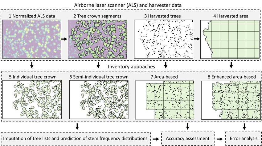
Fig. 1. Study design to compare four inventory approaches for imputing stand-level distributions of stem diameter, tree height, volume and sawn wood volume using harvester and ALS data. We assessed the accuracies of the approaches by comparing the imputed distributions with reference distributions recorded by the harvester, as well as stand mean values. We further assessed which factors influenced the obtained errors.
We segmented trees from the ALS data and delineated harvested areas from the harvester data. We tessellated polygons of harvested areas using a regular grid of 250 m2 and used grid cells that were located completely within those polygons as ABA harvester plots. We then used polygons of segmented tree crowns that intersected ABA grid cells to adjust cell borders to obtain EABA plots. We used the same tree crown segments as observations for the ITC and semi-ITC approaches. For the ITC approach, we spatially joined harvested trees of which the coordinates of the tree top (x,y,z) in the harvester data were nearest to the coordinates of the tree top detected in the ALS data. For the semi-ITC approach, we spatially joined all trees to their nearest tree crown segment. We computed ALS metrics for all ABA and EABA plots and tree crown segments.
We used the kNN technique to impute stem frequency distributions of stem diameter, tree height, volume and sawn wood volume from ALS data. In the imputation, individual tree data from nearest neighbors were used to impute stem frequencies within class values of the studied forest attributes. We compared the imputed distributions with observed distributions recorded by the harvester. Finally, we performed an error analysis in which we assessed how the forest attribute, inventory approach, imputation technique, stand size, ALS pulse density, delay between ALS data acquisition and harvesting, and percentage of deciduous trees in the stand influenced errors in imputed distributions.
2.2 Harvester data
We used harvester data collected from 37 harvesting operations in the municipalities Etnedal, Nord-Aurdal, Sør-Aurdal and Nordre Land in southern Norway (Fig. 2). The harvested trees comprised mainly Norway spruce (Picea abies (L.) Karst.), however some Scots pines (Pinus sylvestris L.) were present as well as deciduous trees, mainly birch (Betula pendula Roth and Betula pubescens Ehrh.).
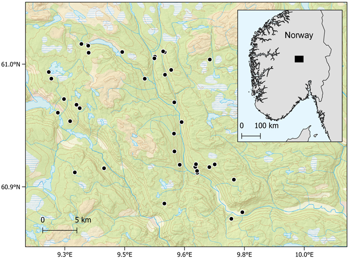
Fig. 2. Locations of harvesting operations in Norway.
The harvester data were collected in the period between March 2019 and June 2021 using a Komatsu 931XC harvester with a 230H crane and a C144 harvester head. The harvester was equipped with a Septentrio AsteRx-U real-time kinematic GNSS comprising two antennas of which positions and rotations were logged at a one second rate in the National Marine Electronics Association (NMEA) format. Locations of harvested trees were recorded with a planimetric accuracy of approximately 1 m, using positions and rotations obtained from the GNSS and the crane extension as measured by sensor hardware (Noordermeer et al. 2021).
Harvester production report (HPR) files were exported after each operation in the StanFord 2010 format (Arlinger et al. 2012). The HPR files included data on tree species, diameter measurements at 10 cm intervals along the stem, log volumes over bark and crane tip coordinates. For each harvested tree, we computed the stem diameter as the diameter (over bark) recorded by the harvester at a length of 110 cm along the stem, the volume as the sum of log volumes (over bark) recorded by the harvester and sawn log volume as the sum of sawn log volumes. Further, because stem profiles only contained data on the processed part of the stem, we predicted the total tree height from the stem profile using taper models (Hansen et al. 2023).
We generated polygons of harvested areas as unary unions of buffers around the positions of harvested stems (Fig. 1, panel 4). We tessellated polygons of harvested areas into grid cells of 250 m2 using a regular grid. The grid size conformed to conventional practices in commercial ALS-based forest inventories in Norway, where sample plots and grid cells of 250 m2 are used in an area-based inventory approach. We defined stands as clusters of grid cells with a minimum total size of 0.2 ha, and that were located completely within the spatial extent of polygons of harvested areas (Fig. 1, panel 7). The minimum size of 0.2 ha conformed to the typical minimum size of forest stands in commercial Norwegian forest inventories. The resulting dataset comprised 49 stands containing 102 289 trees of which 89% were spruce, 7% were pine and 4% were deciduous. Stand sizes ranged from 0.2 to 5.3 ha with a mean of 1.0 ha. A summary of the harvested trees is provided in Table 1.
| Table 1. Summary statistics (mean and range) of stem diameters, tree heights predicted with taper models, volumes (over bark), and sawnwood volumes (over bark) of harvested trees. | |||||
| Species | n | Stem diameter (cm) | Height (m) | Volume (dm3) | Sawnwood volume (dm3) |
| Spruce | 91 237 | 19.5 (5.1–64.0) | 14.9 (2.1–49.9) | 301 (5–4906) | 92 (0–3559) |
| Pine | 7236 | 27.0 (5.3–58.4) | 18.8 (4.8–50) | 603 (14–3602) | 310 (0–2354) |
| Deciduous | 3336 | 16.3 (5.7–63.5) | 14.8 (4.7–53) | 179 (11–4635) | 0 (0–514) |
2.3 Airborne laser scanner data
Four ALS surveys covered the harvested stands, acquired in 2013, 2016, 2017 and 2019 with different instruments and acquisition parameters (Table 2). The ALS data covered different areas which overlapped in some places. The elapsed time between ALS acquisition and harvesting varied from zero to eight years with a mean of five years. The contractors Blom Geomatics AS and Terratec AS processed the raw ALS data and classified laser echoes as ground or non-ground. For each harvesting operation, we used the most recently acquired ALS data. We used the lidR package (Roussel et al. 2020) in R (R Core Team 2022) to construct digital terrain models as triangulated irregular networks (TIN) from the laser echoes classified as ground. We then normalized the ALS data by computing the height relative to the terrain height of the TIN for all echoes.
| Table 2. Airborne laser scanning acquisition parameters, footprint diameters and mean pulse densities. | ||||||||
| Year | Instrument | Time period | Pulse rate (kHz) | Scan rate (Hz) | Flying altitude (m) | Scanning angle (±°) | Footprint diameter (m) | Pulse density (m–2) |
| 2013 | TopEye S/N 444 | May–July | 200 | 92 | 1500 | 20 | 0.28 | 16.4 |
| 2016 | Riegl LMS Q-1560 | September | 400 | 100 | 2900 | 20 | 0.25 | 5.1 |
| 2017 | Riegl VQ-1560 I | July | 700 | 240 | 2300 | 20 | 0.58 | 9.7 |
| 2019 | Leica ALS70-HP | August | 495 | 69 | 1150 | 16 | 0.73 | 29.6 |
2.4 Tree crown segmentation
We generated canopy height models for the harvested stands as rasterized values of maximum ALS height with a spatial resolution of 0.5 m. We located trees in the canopy height models using the locate_trees function of the lidR package, which implements a local maximum filter proposed by Popescu and Wynne (2004), using a window size of 5 m. We then segmented trees from the canopy height model using the dalponte2016 function of the lidR package, using default values. The function implements the segmentation algorithm proposed by Dalponte and Coomes (2016). We computed the height and coordinates (x,y,z) of the highest laser echo within each crown segment. The resulting tree crown polygons represented spatial extents of tree crowns and contained coordinates of treetops detected in the ALS data.
2.5 Polygons of grid cells and tree crown segments
Our analysis required polygons of grid cells, hereafter harvester plots, and tree crown segments as reference and target observations. For the ABA inventory approach, we used the regular grid cells of 250 m2 (Fig. 1, panel 7) as harvester plots, i.e., the grid cells located completely within the spatial extent of polygons of harvested areas. The resulting dataset comprised 2040 harvester plots. For the EABA inventory approach, we used polygons of segmented tree crowns that intersected the ABA plots to adjust plot borders following the approach proposed by Packalén et al. (2015). We merged each tree crown segment with the intersecting ABA plot with which it overlapped most (Fig. 1, panel 8). For the ITC approach, we used the same tree crown segments that intersected the ABA plots, which we spatially joined with the nearest harvested trees. In case of multiple harvested trees being joined with a given tree crown segment, we used the harvested tree of which the coordinates of the tree top (x,y,z) were nearest to the coordinates of the tree top detected in the ALS data. For the semi-ITC approach, we used the same tree crown segments as those used for the ITC approach, and spatially joined them to the nearest harvested tree. However, multiple harvested trees were allowed for a given tree crown segment. Resultingly, some semi-ITC segments were empty, some contained a single tree, and some contained multiple trees. For each inventory approach, we generated tree lists for the harvester plots or tree crown segments.
2.6 Airborne laser scanner metrics
We extracted ALS echoes from within harvester plots and tree crown segments and computed ALS metrics from first (and single) laser echoes. We computed the maximum height, mean height, standard deviation, skewness and kurtsosis. We further computed the percentage of echoes above the mean height and 2 m, and the normalized Shanon diversity index proposed by van Ewijk et al. (2011). We computed echo heights at the 10th, 20th, …, 90th percentiles of the height distributions as well as the 95th percentile. Finally, we divided the height range between the lowest canopy echo > 2 m and the 95th percentile into 10 fractions of equal height and computed canopy density metrics (D0, D1, …, D9) as the proportion of echoes above each fraction divided by the total number of echoes.
2.7 Imputation of stem frequency distributions
We imputed stand-level distributions of stem diameter, tree height, volume and sawn wood volume from the ALS data using the four inventory approaches: ITC, semi-ITC, ABA, and EABA. We used the kNN technique to impute tree lists for each target observation based on the nearest neighbors, i.e., observations in the reference data of which a selection of ALS metrics were most similar to the corresponding ALS metrics of the target observation. We applied three-fold spatial cross validation, whereby we removed one third of the stands at a time as target data and used the remaining stands as reference data. We assigned spatially close stands to the same folds using k-means clustering. For each fold, we imputed tree lists for target observations using the Euclidean distance metric. We then selected ALS metrics as predictor variables and determined the number of nearest neighbors. In the following sections, the methods used for the imputation are explained in depth.
2.7.1 Nearest neighbor imputation
When nearest neighbor techniques are used for imputation, predictor variables should be selected to determine the similarity between pairs of observations (McRoberts et al. 2015). We used the leaps package (Lumley 2004) for the selection of ALS metrics as predictor variables for each of the four studied forest attributes separately. We used the regsubsets function to find optimal subsets of predictor variables for linear regression models with stem diameter, tree height, volume and sawn wood volume as response variables. We used exhaustive search and set a maximum of five predictor variables in each subset. We used the caret package (Kuhn 2008) to select the number of neighbors, k, for the four forest attributes separately. We used potential values of k = 5, 7, …, 15, and selected the value of k that minimized the root mean square error. We then used the yaImpute package (Crookston and Finley 2008) in R to identify the k-nearest neighbors in the reference data, based on the selected ALS metrics and k.
2.7.2 Removal of potentially erroneous reference data
A preliminary analysis revealed possible co-location errors between harvester and ALS data, i.e., harvester plots and tree crown segments of which ALS heights differed substantially from the heights of harvested trees (Fig. 3). Such large deviations in height may have been caused by errors in the harvester data or temporal decorrelation caused by the delay between ALS acquisition and harvesting. We identified and excluded such observations in the reference data prior to the imputation, similar to methods used by Breidenbach et al. (2010). We fitted a simple linear regression model with the maximum tree height obtained from the harvester data as the response variable and the 95th percentile of ALS height as the predictor variable. We then labeled those observations in the reference data that had a Cooks distance > 0.5 of the mean Cooks distance as erroneous. We removed erroneous observations only from the reference data, i.e., not from the target data, prior to the nearest neighbor imputation in each fold.
2.7.3 Imputation of tree lists
We imputed sets of trees for target observations following the methods described by Packalén and Maltamo (2008):
![]()
where Tuj is a set of trees imputed for the target observation j based on k reference observations denoted u, each containing 1, 2, …, n trees. For example, ![]() is the first tree of the first reference observation used for imputation for target observation j. We computed the similarities between each target observation and the selected k-nearest neighbors in the reference data, as the inverse of the distance matrices. We then used the similarities as weights in imputing the resultant tree lists for target observations:
is the first tree of the first reference observation used for imputation for target observation j. We computed the similarities between each target observation and the selected k-nearest neighbors in the reference data, as the inverse of the distance matrices. We then used the similarities as weights in imputing the resultant tree lists for target observations:
![]()
where Tj is the imputed tree list for target observation j and Wkj is the similarity between reference observation u and target observation j. Thus, each stem frequency in each class of a reference observation was weighted with the similarity between the target and reference observation. For each target observation, we obtained an imputed stem frequency for each class within the distributions of the studied forest attributes. The classes covered the range of the observed tree attributes in the harvester data, divided into 20 intervals of equal size for all the studied attributes. Finally, from the stand-wise imputed tree lists, we estimated the mean stem diameter, tree height, volume, sawn wood volume and number of stems for each stand, which in the latter three cases we scaled to a per ha unit.
2.8 Accuracy assessment
We compared the imputed distributions with observed distributions obtained from the harvester data at stand level. Because the harvested trees included in ABA and EABA plots differed slightly in some cases due to differences in cell borders (Fig. 1), the observed distributions were computed for the two approaches separately. The observed distributions obtained for the EABA approach also served as observed distributions for the ITC and semi-ITC approaches because the spatial extent of tree crown segments corresponded, and the trees included in the reference data were thus identical. We assessed the accuracies of imputed distributions for each stand using an error index (EI) proposed by Packalén and Maltamo (2008):

where c is the number of classes in the frequency distribution, fi is the reference stem frequency within class i, ![]() is the corresponding imputed stem frequency, N is the reference number of stems within all classes and
is the corresponding imputed stem frequency, N is the reference number of stems within all classes and ![]() is the imputed number of stems within all classes. The EI ranges from 0to 1 and is inversely proportional to accuracy, i.e., a lower value implies better accuracy.
is the imputed number of stems within all classes. The EI ranges from 0to 1 and is inversely proportional to accuracy, i.e., a lower value implies better accuracy.
We further assessed the accuracies of stand mean estimates using the root mean square error relative to the mean:

where n is the number of stands, Xi is the observed stand-level forest attribute in stand i, ![]() is the corresponding estimated forest attribute, and
is the corresponding estimated forest attribute, and ![]() is the mean value of the studied forest attribute for all stands. We further computed the mean difference between observed and estimated values, relative to the mean:
is the mean value of the studied forest attribute for all stands. We further computed the mean difference between observed and estimated values, relative to the mean:

2.9 Error analysis
We assessed whether the errors obtained for the imputed distributions could be explained by the forest attribute, inventory approach, imputation technique, stand size, pulse density, number of years between ALS and harvester data acquisition (ALS delay), or the percentage of deciduous trees (%Deciduous). We fitted a linear model with the stand-wise EI obtained for all forest attributes, inventory approaches, and imputation techniques as the response, and the forest attribute, inventory approach, stand size, pulse density, ALS delay, and percentage of deciduous trees as predictor variables. The data used for the modelling were characterized by a hierarchical structure whereby error indices were repeated measurements for stands. We accounted for this dependency by fitting a mixed model with a random intercept for the stand. We fitted the model using the lme4 package (Bates et al. 2015) in R. We selected the following model form based on model diagnostics and analysis of variance comparisons:
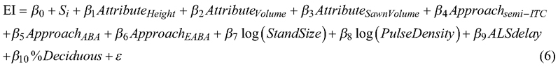
where Si is the random intercept for stand i, β0,1, ... ,10 are parameters to be estimated, AttributeHeight, AttributeVolume, and AttributeSawnVolume are indicator variables representing the forest attributes tree height, volume and sawn wood volume, respectively, where stem diameter is the baseline, ApproachITC, Approachsemi-ITC , and ApproachEABA are indicator variables representing the inventory approaches ITC, semi-ITC and EABA, respectively, where ABA is the baseline, StandSize is the stand size in ha, PulseDensity is the mean number of laser pulses per m2 in the stand, ALSdelay is the number of years between ALS and harvester data acquisition, %Deciduous is the percentage of deciduous trees in the stand and ε is the model error. We tested whether the predictor variables significantly influenced the error indices by constructing 95% confidence intervals of parameter estimates from the likelihood profile. Further, we assessed how the predictor variables affected the stand-level error indices based on estimates obtained for β7–β10.
3 Results
3.1 Imputation of stem frequency distributions
Fig. 3 shows an example of observations used as reference data in the imputation and observations labeled as erroneous and therefore not used for nearest neighbor imputation. The percentage of trees labeled as erroneous ranged from 20% to 32% for the four inventory approaches and three folds. The number of nearest neighbors selected for the four inventory approaches and in the three folds ranged from 11 to 15 with a mean of 13.
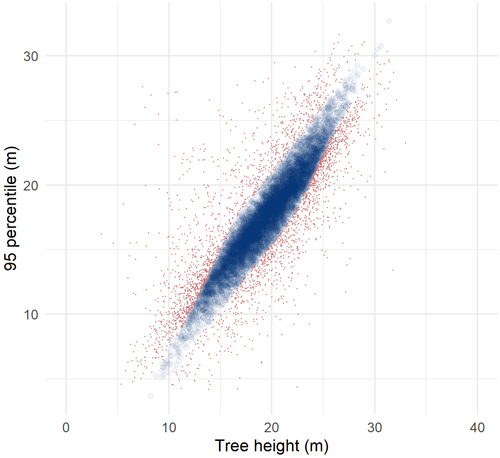
Fig. 3. Heights of harvested trees plotted against the 95 percentile of laser echo heights for observations in the reference data used for an example fold and the individual tree crown approach. Observations used as reference data in the imputation are shown as transparent blue circles and observations labeled as erroneous are shown as red dots.
Error indices obtained for the stand-wise imputed distributions for the four inventory approaches are shown in Fig. 4. We obtained smallest error indices for imputation of volume distributions using the semi-ITC, ABA, and EABA inventory approaches. Error indices were similar across forest attributes. We obtained best accuracies, i.e., smallest values of EI, of 0.13, 0.13, 0.10 and 0.10, for distributions of stem diameter, tree height, volume, and sawn wood volume.
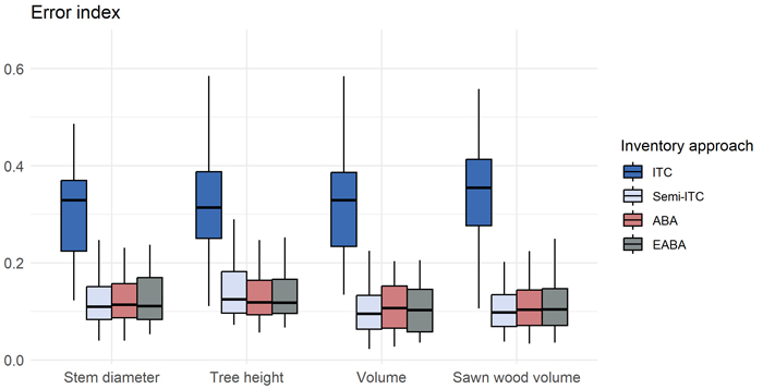
Fig. 4. Box plot of error indices obtained for stand-level imputed distributions of the studied attributes, obtained for the four inventory approaches: individual tree crown (ITC), semi-ITC, area-based approach (ABA) and enhanced ABA.
Fig. 5 shows reference and imputed distributions of the four attributes for a representative example stand. Distributions imputed following the ITC approach showed systematic errors, with underpredicted stem frequencies in smaller classes. Imputed stem frequencies obtained for the remaining inventory approaches tended to be similar.
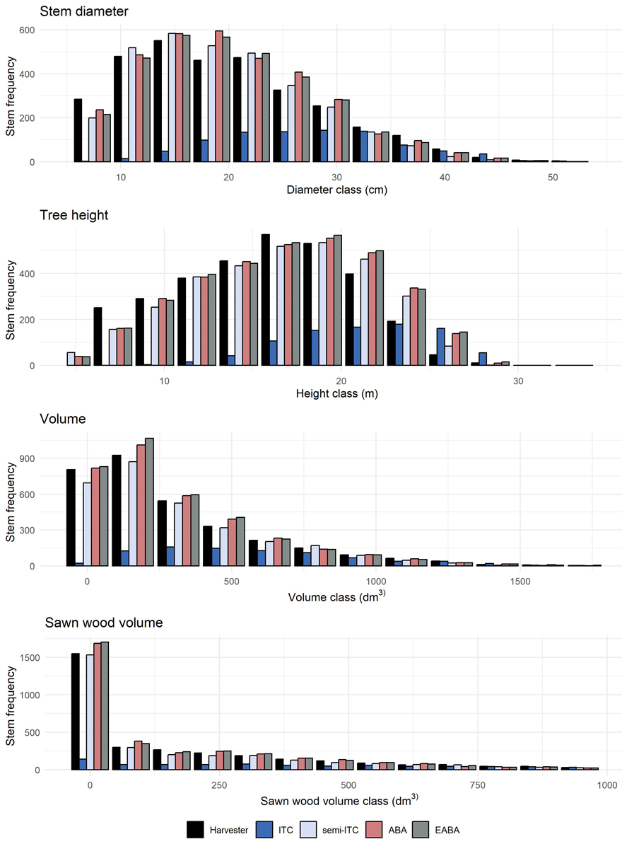
Fig. 5. Imputed stem frequency distributions obtained for a representative example stand, i.e., with an error index nearest to the mean error index obtained for all stands, recorded by the harvester and imputed using the four inventory approaches: individual tree crown (ITC), semi-ITC, area-based approach (ABA) and enhanced ABA (EABA).
3.2 Estimation of stand-level forest attributes
The results of the stand-level estimation of mean values are shown in Table 3. Values of RMSE% obtained for the ITC approach were substantially better than those obtained for the remaining approaches. Apart from the ITC approach, values of MD%, i.e., systematic errors, were < 10% for stand mean estimates of all forest attributes. Overall, the semi-ITC approach gave the best mean accuracies.
| Table 3. Errors obtained for estimates of stand-level forest attributes, as root mean square errors and mean differences relative to the observed mean values (RMSE%, MD%), for the four inventory approaches: individual tree crown (ITC), semi-ITC, area-based approach (ABA) and enhanced ABA (EABA). | ||||||||
| ITC | Semi-ITC | ABA | EABA | |||||
| RMSE% | MD% | RMSE% | MD% | RMSE% | MD% | RMSE% | MD% | |
| Stem diameter (cm) | 30.1 | –24.4 | 14.6 | 5.7 | 14.6 | 4.7 | 15.2 | 4.9 |
| Height (m) | 22.2 | –18.0 | 9.1 | 3.6 | 8.9 | 1.8 | 8.7 | 1.2 |
| Volume (m3 ha–1) | 66.9 | 52.5 | 13.6 | 3.1 | 19.0 | 1.7 | 16.6 | 2.8 |
| Sawn wood volume (m3 ha–1) | 65.0 | 42.9 | 19.7 | 2.5 | 21.2 | 3.1 | 21.3 | 2.0 |
| Number of stems (ha–1) | 75.3 | 70.6 | 17.4 | –2.7 | 22.1 | –3.9 | 21.7 | –5.1 |
3.3 Error analysis
The results of the fitted model used in the error analysis (Eq. 6) are shown in Fig. 6. The forest attribute, inventory approach, stand size and the laser pulse density significantly influenced the stand-level EI (p < 0.05). On average, values of EI increased by 20.4 when the ITC approach was used, in comparison to the baseline which was the ABA approach. Values of EI obtained for the semi-ITC and EABA approaches did not differ significantly from the ABA approach. Increased ALS delay and the percentage of deciduous trees in the stand did not cause larger errors in imputed frequency distributions.
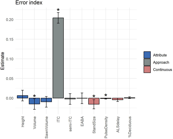
Fig. 6. Parameter estimates (bars) and 95% confidence intervals (whiskers) obtained for the fitted model used in the error analysis. Variables that significantly influenced the obtained error indices (p < 0.05) are labeled with an asterisk.
4 Discussion
Stem frequency distributions can provide detailed information useful for pre-harvest forest planning. We compared four inventory approaches for imputation of stem frequency distributions by four forest attributes. We further assessed which factors influenced the accuracy of the imputed distributions.
Most previous studies on predicting distributions from ALS data have focused on stem diameter distributions and used conventional field plot measurements as reference data. For example, Packalén and Maltamo (2008) predicted species-specific stem diameter distributions and compared nearest neighbor imputation with parameter estimation of a theoretical (Weibull) distribution. The nearest neighbor technique outperformed the parametric technique, and they obtained values of EI of 0.33 and 0.21 in predicting Norway spruce stem diameter distributions, for the two approaches, respectively. We obtained better accuracies for imputed stem diameter distributions in this study, i.e., a mean EI of 0.13 obtained for the semi-ITC, ABA and EABA approaches. This may have been due to the relatively large numbers of reference observations used in this study, i.e., 2040 harvester plots and 11 975 tree crown segments, in comparison to <500 field plots used in the mentioned study. In addition, the mentioned study used data comprising various stand development classes and a mixture of species, as opposed to mature spruce stands ready for harvest. Furthermore, the mentioned study used data collected from an average of seven plots per stand, while we used harvester data which comprised entire stands. In another study, Söderberg et al. (2021) used harvester data from clear-felled stands and ALS data to impute diameter distributions at stand level. Indeed, that study reported values of EI of 0.13–0.14, i.e., equivalent to the level of accuracy obtained here.
Maltamo et al. (2019) imputed stand-level stem diameter distributions using harvester reference data and the kNN technique. The study reported better accuracies than previous studies using field plot data; values of EI ranged from 0.15 to 0.19, depending on the size of the ABA harvester plots used in the reference data, however 0.15 when a plot size of 200 m2 was used and comparable to our plot size of 250 m2. In this study, we obtained a similar level of accuracy, i.e., mean EI of 0.13 obtained for the ABA, EABA and semi-ITC inventory approaches, confirming the accuracy reported in the mentioned study.
Accuracies of imputed distributions of tree height, volume and sawn wood volume were similar to, or better than, accuracies obtained for imputed distributions of stem diameter (Fig. 4). This result highlights the utility of harvester and ALS data for imputing distributions of forest attributes other than stem diameter. In a previous study on predicting stand-level top diameter distributions of sawlogs using harvester and ALS data, Barth et al. (2015) obtained values of EI of 0.34 and 0.15 for all diameter classes and diameter classes ≥15 cm, respectively. The mentioned study demonstrated the utility of harvester data as reference data in predicting product recovery in logging operations. In another study, however, Mehtätalo et al. (2015) used ALS data to predict plot-wise distributions of tree height using a parametric approach. The study reported unsatisfactory results based on comparisons of the predicted distributions with empirical data and therefore advised against practical use of the method.
We obtained significantly poorer accuracies for the ITC approach compared to other inventory approaches. This result confirms findings of previous studies in that the ITC approach can lead to systematic errors due to trees not being detected in the ALS data and thus missing in the reference data (Breidenbach et al. 2010; Maltamo et al. 2004). Smaller trees are less likely to be detected and delineated from the ALS data, and resultingly, smaller trees are typically missing in the imputed distributions (Bergseng et al. 2015). In previous studies assessing tree detection from ALS data, detection rates have varied considerably and typically ranged between 25% and 80% (Kaartinen et al. 2012). The detection rate has been found to be strongly affected by forest structure (Falkowski et al. 2008; Vauhkonen et al. 2012). In this study, a total of 43 371 trees were segmented from the ALS data within the harvested stands, while the harvester data comprised 102 289 trees within the corresponding areas, i.e., a detection rate of 42%. Thus, these trees not detected in the reference data are likely the main cause of the relatively poor results obtained for the ITC approach.
Error indices obtained for distributions imputed using the semi-ITC and ABA inventory approaches were similar for most forest attributes, as well as errors in stand-level estimates of those attributes. This result was in accordance with findings from Rahlf et al. (2015) who compared the two approaches in predicting forest attributes from image-based point cloud data, and obtained similar accuracies for the two approaches. By accounting for edge effects along harvester plot borders, we assessed whether the EABA would result in better accuracies than the ABA. The error analysis revealed that this was not the case. This finding contrasted with earlier studies that showed that by resolving edge effects and co-location errors between reference data and ALS data, better accuracies can be obtained using an EABA (Packalén et al. 2015; Pascual 2019).
In previous studies, the integration of ITC and ABA approaches has yielded promising results for ALS-based imputation of tree-level data (Breidenbach et al. 2012; Lindberg et al. 2010). In a study on predicting stem diameter distributions from ALS data, Xu et al. (2014) found that combining the ITC and ABA approaches can improve the accuracy of predicted distributions. The study compared two methods, namely (1) replacement, whereby large diameter classes in ABA-derived distributions were replaced by ITC-derived trees, and (2) by matching histograms obtained with ABA and ITC. The best accuracy was obtained by the second approach, whereby the accuracy of predicted distributions only increased slightly due to the ITC-derived information.
Our findings demonstrate that harvester data can be linked to ALS data to impute stem frequency distributions of forest attributes other than stem diameter with satisfactory accuracy. This suggests the potential applicability of the proposed methods in ALS-based inventories. However, harvester data primarily comprise mature forest stands ready for harvest. This can introduce sampling biases, and, consequently, lead to systematic errors in forest inventory based on harvester data, as demonstrated by Räty et al. (2022). Their study revealed that harvester data proved more useful in productive forests than unproductive forests, although they reported systematic errors in both cases. The study also showed that such systematic errors could be mitigated when a probability sample of field measurements obtained from sample plots is available within the inventory area. Thus, while the methods proposed here show promise in pre-harvest inventory of mature forest stands, operational application of the methods in other forest types may require supplementary sample plot data for unbiased results. Therefore, further research is needed to assess whether the methods are applicable to more variable forest types, potentially supported by samples of field plots typically used in conventional ALS-based inventories.
5 Conclusions
This study highlights the utility of harvester and ALS data for imputing stem frequency distributions in mature spruce-dominated stands. The choice of inventory approach had great impact on the accuracies of the imputed distributions. We obtained significantly better accuracies for the semi-ITC, ABA and EABA inventory approaches than the ITC approach. The forest attribute, inventory approach, stand size and the laser pulse density had significant effects on the accuracies of imputed frequency distributions, however the ALS delay and percentage of deciduous trees did not.
Declaration of openness of research materials, data, and code
The harvester data used in this study are owned by the contractor, Valdres Skog AS, and therefore not openly available. The ALS data are available at https://hoydedata.no. The statistical code is available upon request.
Author contributions
Conceptualization: L.N., T.G.; Data curation: L.N.; Formal analysis: L.N., H.O.; Funding acquisition: T.G.; Methodology: L.N.; Validation: L.N.; Visualization: L.N.; Writing – original draft: L.N.; Writing – review & editing: L.N., H.O., T.G.
Funding
This work is part of the Center for Research-based Innovation SmartForest: Bringing Industry 4.0 to the Norwegian forest sector (NFR SFI project no. 309671, smartforest.no).
Acknowledgements
We wish to thank Valdres Skog AS for collecting the harvester data. We further extend our thanks to Blom Geomatics AS and Terratec AS for collecting and processing the ALS data, and Komatsu Forestry AB and Gundersen & Løken AS for their technical support. We also thank the reviewers for their useful comments and suggestions.
References
Arlinger J, Nordström M, Möller, JJ (2012) StanForD 2010: modern communication with forest machines. Report nr 785, Skogforsk.
Bates D, Mächler M, Bolker B, Walker S (2015) Fitting linear mixed-effects models using lme4. J Stat Softw 67: 1–48. https://doi.org/10.18637/jss.v067.i01.
Barth A, Möller JJ, Wilhelmsson L, Arlinger J, Hedberg R, Söderman U (2015) A Swedish case study on the prediction of detailed product recovery from individual stem profiles based on airborne laser scanning. Ann For Sci 72: 47–56. https://doi.org/10.1007/s13595-014-0400-6.
Bergseng E, Ørka HO, Næsset E, Gobakken T (2015) Assessing forest inventory information obtained from different inventory approaches and remote sensing data sources. Ann For Sci 72: 33–45. https://doi.org/10.1007/s13595-014-0389-x.
Brandtberg T (1999) Automatic Individual tree-based analysis of high spatial resolution remotely sensed data. PhD thesis. Acta Universitatis Agriculutae Sueciae, Sivestria 118. Swedish University of agricultural Sciences, Uppsala.
Breidenbach J, Næsset E, Lien V, Gobakken T, Solberg S (2010) Prediction of species specific forest inventory attributes using a nonparametric semi-individual tree crown approach based on fused airborne laser scanning and multispectral data. Remote Sens Environ 114: 911–924. https://doi.org/10.1016/j.rse.2009.12.004.
Breidenbach J, Næsset E, Gobakken T (2012) Improving k-nearest neighbor predictions in forest inventories by combining high and low density airborne laser scanning data. Remote Sens Environ 117: 358–365. https://doi.org/10.1016/j.rse.2011.10.010.
Cover T, Hart P (1967) Nearest neighbor pattern classification. IEEE Trans Inf Theory 13: 21–27. https://doi.org/10.1109/tit.1967.1053964.
Crookston NL, Finley AO (2008) yaImpute: an R package for kNN imputation. J Stat Softw 23: 1–16. https://doi.org/10.18637/jss.v023.i10.
Dalponte M, Coomes DA (2016) Tree‐centric mapping of forest carbon density from airborne laser scanning and hyperspectral data. Meth Ecol Evol 7: 1236–1245. https://doi.org/10.1111/2041-210x.12575.
Dalponte M, Frizzera L, Ørka HO, Gobakken T, Næsset E, Gianelle D (2018) Predicting stem diameters and aboveground biomass of individual trees using remote sensing data. Ecol Indic 85: 367–376. https://doi.org/10.1016/j.ecolind.2017.10.066.
Duvemo K, Lämås T (2006) The influence of forest data quality on planning processes in forestry. Scand J For Res Research 21: 327–339. https://doi.org/10.1080/02827580600761645.
Eid T, Hobbelstad K (2000) AVVIRK-2000: a large-scale forestry scenario model for long-term investment, income and harvest analyses. Scand J For Res 15: 472–482. https://doi.org/10.1080/028275800750172736.
Falkowski MJ, Smith AM, Gessler PE, Hudak AT, Vierling LA, Evans JS (2008) The influence of conifer forest canopy cover on the accuracy of two individual tree measurement algorithms using lidar data. Can J Remote Sens 34: 338–350. https://doi.org/10.5589/m08-055.
Gobakken T, Næsset E (2004) Estimation of diameter and basal area distributions in coniferous forest by means of airborne laser scanner data. Scand J For Res 19: 529–542. https://doi.org/10.1080/02827580410019454.
Hansen E, Rahlf J, Astrup R, Gobakken T (2023) Taper, volume, and bark thickness models for spruce, pine, and birch in Norway. Scand J For Res 38: 413–428. https://doi.org/10.1080/02827581.2023.2243821.
Hauglin M, Hansen EH, Næsset E, Busterud BE, Gjevestad JGO, Gobakken T (2017) Accurate single-tree positions from a harvester: a test of two global satellite-based positioning systems. Scand J For Res 32: 774–781. https://doi.org/10.1080/02827581.2017.1296967.
Hyyppä J (1999) Detecting and estimating attributes for single trees using laser scanner. Photogramm J Finland 16: 27–42.
Kaartinen H, Hyyppä J, Yu X, Vastaranta M, Hyyppä H, Kukko A, Holopainen M, Heipke C, Hirschmugl M, Morsdorf F (2012) An international comparison of individual tree detection and extraction using airborne laser scanning. Remote Sens 4: 950–974. https://doi.org/10.3390/rs4040950.
Kandare K, Dalponte M, Ørka HO, Frizzera L, Næsset E (2017) Prediction of species-specific volume using different inventory approaches by fusing airborne laser scanning and hyperspectral data. Remote Sens 9, article id 400. https://doi.org/10.3390/rs9050400.
Kemmerer J, Labelle ER (2020) Using harvester data from on-board computers: a review of key findings, opportunities and challenges. Eur J For Res 140: 1–17. https://doi.org/10.1007/s10342-020-01313-4.
Kuhn M (2008) Building predictive models in R using the caret package. J Stat Softw 28: 1–26. https://doi.org/10.18637/jss.v028.i05.
Kuuluvainen T, Penttinen A, Leinonen K, Nygren M (1996) Statistical opportunities for comparing stand structural heterogeneity in managed and primeval forests: an example from boreal spruce forest in southern Finland. Silva Fenn 30: 315–328. https://doi.org/10.14214/sf.a9243.
Lindberg E, Holmgren J, Olofsson K, Wallerman J, Olsson H (2010) Estimation of tree lists from airborne laser scanning by combining single-tree and area-based methods. Int J Remote Sens 31: 1175–1192. https://doi.org/10.1080/01431160903380649.
Lindroos O, Ringdahl O, La Hera P, Hohnloser P, Hellström TH (2015) Estimating the position of the harvester head – a key step towards the precision forestry of the future? Croat J For Eng 36: 147–164.
Lumley T (2004) The leaps package for regression subset selection. R package version 2.9.
Maltamo M, Mustonen K, Hyyppä J, Pitkänen J, Yu X (2004) The accuracy of estimating individual tree variables with airborne laser scanning in a boreal nature reserve. Can J For Res 34: 1791–1801. https://doi.org/10.1139/x04-055.
Maltamo M, Eerikäinen K, Packalén P, Hyyppä J (2006) Estimation of stem volume using laser scanning-based canopy height metrics. Forestry 79: 217–229. https://doi.org/10.1093/forestry/cpl007.
Maltamo M, Næsset E, Vauhkonen J (2014) Forestry applications of airborne laser scanning. Concepts and case studies. Manag For Ecosyst 27, article id 460. https://doi.org/10.1007/978-94-017-8663-8_1.
Maltamo M, Hauglin M, Næsset E, Gobakken T (2019) Estimating stand level stem diameter distribution utilizing harvester data and airborne laser scanning. Silva Fenn 53, article id 10075. https://doi.org/10.14214/sf.10075.
McRoberts RE, Næsset E, Gobakken T (2015) Optimizing the k-nearest neighbors technique for estimating forest aboveground biomass using airborne laser scanning data. Remote Sens Environ 163: 13–22. https://doi.org/10.1016/j.rse.2015.02.026.
Mehtätalo L, Maltamo M, Packalen P (2007) Recovering plot-specific diameter distribution and height-diameter curve using ALS based stand characteristics. ISPRS Workshop on Laser Scanning and SilviLaser, pp 288–293. https://api.semanticscholar.org/CorpusID:18875433.
Mehtätalo L, Virolainen A, Tuomela J, Packalen P (2015) Estimating tree height distribution using low-density ALS data with and without training data. IEEE J Sel Top Appl Earth Obs Remote Sens 8: 1432–1441. https://doi.org/10.1109/jstars.2015.2418675.
Næsset E (2002) Predicting forest stand characteristics with airborne scanning laser using a practical two-stage procedure and field data. Remote Sens Environ 80: 88–99. https://doi.org/10.1016/s0034-4257(01)00290-5.
Næsset E, Bollandsås OM, Gobakken T, Gregoire TG, Ståhl G (2013) Model-assisted estimation of change in forest biomass over an 11 year period in a sample survey supported by airborne LiDAR: a case study with post-stratification to provide “activity data”. Remote Sens Environ 128: 299–314. https://doi.org/10.1016/j.rse.2012.10.008.
Noordermeer L, Sørngård E, Astrup R, Næsset E, Gobakken T (2021) Coupling a differential global navigation satellite system to a cut-to-length harvester operating system enables precise positioning of harvested trees. Int J For Eng 32: 119–127. https://doi.org/10.1080/14942119.2021.1899686.
Packalén P, Maltamo M (2008) Estimation of species-specific diameter distributions using airborne laser scanning and aerial photographs. Can J For Res 38: 1750–1760. https://doi.org/10.1139/x08-037.
Packalén P, Strunk JL, Pitkänen JA, Temesgen H, Maltamo M (2015) Edge-tree correction for predicting forest inventory attributes using area-based approach with airborne laser scanning. IEEE J-STARS 8: 1274–1280. https://doi.org/10.1109/jstars.2015.2402693.
Pascual A (2019) Using tree detection based on airborne laser scanning to improve forest inventory considering edge effects and the co-registration factor. Remote Sens 11, article id 2675. https://doi.org/10.3390/rs11222675.
Persson A, Holmgren J, Soderman U (2002) Detecting and measuring individual trees using an airborne laser scanner. Photogramm Eng Remote Sens 68: 925–932.
Peuhkurinen J, Maltamo M, Malinen J, Pitkänen J, Packalén P (2007) Preharvest measurement of marked stands using airborne laser scanning. For Sci 53: 653–661. https://doi.org/10.1093/forestscience/53.6.653.
Peuhkurinen J, Maltamo M, Malinen J (2008) Estimating species-specific diameter distributions and saw log recoveries of boreal forests from airborne laser scanning data and aerial photographs: a distribution-based approach. Silva Fenn 42: 625–641. https://doi.org/10.14214/sf.237.
Peuhkurinen J, Mehtätalo L, Maltamo M (2011) Comparing individual tree detection and the area-based statistical approach for the retrieval of forest stand characteristics using airborne laser scanning in Scots pine stands. Can J For Res 41: 583–598. https://doi.org/10.1139/x10-223.
Popescu SC, Wynne RH (2004) Seeing the trees in the forest: using lidar and multispectral data fusion with local filtering and variable window size for estimating tree height. Photogramm Eng Remote Sens 70: 589–604. https://doi.org/10.14358/PERS.70.5.589.
R Core Team (2022) A language and environment for statistical computing. https://www.R-project.org/.
Rahlf J, Breidenbach J, Solberg S, Astrup R (2015) Forest parameter prediction using an image-based point cloud: a comparison of semi-ITC with ABA. Forests 6: 4059–4071. https://doi.org/10.3390/f6114059.
Räty J, Packalen P, Maltamo M (2018) Comparing nearest neighbor configurations in the prediction of species-specific diameter distributions. Ann For Sci 75: 1–16. https://doi.org/10.1007/s13595-018-0711-0.
Räty J, Hauglin M, Astrup R, Breidenbach J (2022) Assessing and mitigating systematic errors in forest attribute maps utilizing harvester and airborne laser scanning data. Can J For Res 53: 284–301. https://doi.org/10.1139/cjfr-2022-0053.
Reynolds MR, Burk TE, Huang WC (1988) Goodness-of-fit tests and model selection procedures for diameter distribution models. For Sci 34: 373–399. https://doi.org/10.1093/forestscience/34.2.373.
Roussel JR, Auty D, Coops NC, Tompalski P, Goodbody TR, Meador AS, Bourdon JF, De Boissieu F, Achim A (2020) lidR: an R package for analysis of Airborne Laser Scanning (ALS) data. Remote Sens Environ 251, article id 112061. https://doi.org/10.1016/j.rse.2020.112061.
Saad R, Wallerman J, Lämås T (2015) Estimating stem diameter distributions from airborne laser scanning data and their effects on long term forest management planning. Scand J For Res 30: 186–196. https://doi.org/10.1080/02827581.2014.978888.
Shang C, Treitz P, Caspersen J, Jones T (2017) Estimating stem diameter distributions in a management context for a tolerant hardwood forest using ALS height and intensity data. Can J Remote Sens 43: 79–94. https://doi.org/10.1080/07038992.2017.1263152.
Söderberg J, Wallerman J, Almäng A, Möller JJ, Willén E (2021). Operational prediction of forest attributes using standardised harvester data and airborne laser scanning data in Sweden. Scand J For Res 36: 306–314. https://doi.org/10.1080/02827581.2021.1919751.
Solberg S, Naesset E, Bollandsas OM (2006) Single tree segmentation using airborne laser scanner data in a structurally heterogeneous spruce forest. Photogramm Eng Remote Sens 72: 1369–1378. https://doi.org/10.14358/pers.72.12.1369.
Thomas V, Oliver R, Lim K, Woods M (2008) LiDAR and Weibull modeling of diameter and basal area. For Chron 84: 866–875. https://doi.org/10.5558/tfc84866-6.
Tompalski P, Coops NC, White JC, Wulder MA (2015) Enriching ALS-derived area-based estimates of volume through tree-level downscaling. Forests 6: 2608–2630. https://doi.org/10.3390/f6082608.
Uuttera J, Maltamo M (1995) Impact of regeneration method on stand structure prior to first thinning. Silva Fenn 29: 267–285. https://doi.org/10.14214/sf.a9213.
van Ewijk KY, Treitz PM, Scott NA (2011) Characterizing forest succession in Central Ontario using LiDAR-derived indices. Photogramm Eng Remote Sens 77: 261–269. https://doi.org/10.14358/pers.77.3.261.
Vauhkonen J, Ene L, Gupta S, Heinzel J, Holmgren J, Pitkänen J, Solberg S, Wang Y, Weinacker H, Hauglin M (2012) Comparative testing of single-tree detection algorithms under different types of forest. Forestry 85: 27–40. https://doi.org/10.1093/forestry/cpr051.
Wikström P, Edenius L, Elfving B, Eriksson LO, Lämås T, Sonesson J, Öhman K, Wallerman J, Waller C, Klintebäck F (2011) The Heureka forestry decision support system: an overview. Math Comput For Nat Resour Sci 3: 87–94.
Xu Q, Hou Z, Maltamo M, Tokola T (2014) Calibration of area based diameter distribution with individual tree based diameter estimates using airborne laser scanning. ISPRS J Photogramm Remote Sens 93: 65–75. https://doi.org/10.1016/j.isprsjprs.2014.03.005.
Total of 61 references.
