Heikki Astola  ,
Annika Kangas,
Francesco Minunno,
Matti Mõttus
,
Annika Kangas,
Francesco Minunno,
Matti Mõttus
Emulating a forest growth and productivity model with deep learning
Astola H., Kangas A., Minunno F., Mõttus M. (2026). Emulating a forest growth and productivity model with deep learning. Silva Fennica vol. 60 no. 1 article id 25012. https://doi.org/10.14214/sf.25012
Highlights
- Emulating the operation of analytical forest growth models is feasible using state-of-the-art machine learning methods
- Long term prediction of forest growth and carbon balance variables were produced with low bias accumulation when compared to the reference model
- The methods tested offer means for long time span simulations of large areas with a high spatial resolution.
Abstract
We studied the possibility of replacing a complex forest growth and productivity model with a deep learning model with sufficient accuracy. We used three different neural network architectures for emulating the prediction task of the PREBASSO (Mäkelä 1997; Minunno et al. 2016) forest growth model: 1) Recurrent Neural Network (RNN) Encoder-decoder network, 2) RNN encoder network, and 3) Transformer encoder network. The PREBASSO forest growth model was used to produce 25-year predictions for forest variables: tree height, stem diameter, basal area, and the carbon balance variables: net primary production (NPP), gross primary production per tree layer (GPP), net ecosystem exchange (NEE) and gross growth (GGR) to train the machine learning models. The Finnish Forest Centre provided the data for 29 619 field inventory plots in continental Finland that were used as the initial state of the forest sites to be simulated. Climate data downloaded from Copernicus Climate Data Store were used to provide realistic climate scenarios. We emphasized the importance of low bias in long term predictions and set the goal for the emulator prediction relative bias to be within ±2%. The RNN encoder model produced the best results with the mean of the yearly bias values within the specified ±2% limit over the 25-year prediction period. The study shows that emulating the operation of analytical forest growth models is feasible using state-of-the-art machine learning methods and indicates the potential of using such emulators for producing long time span simulations for e.g. digital twins.
Keywords
carbon balance;
simulation;
machine learning;
climate scenarios;
digital twins;
forest variables;
time series prediction
-
Astola,
VTT Technical Research Centre of Finland, Tekniikantie 1, 02150 Espoo, Finland
 https://orcid.org/0000-0003-4989-9910
E-mail
heikki.astola@gmail.com
https://orcid.org/0000-0003-4989-9910
E-mail
heikki.astola@gmail.com
-
Kangas,
Natural Resources Institute Finland (Luke), Bioeconomy and Environment, Yliopistokatu 6, 80100 Joensuu, Finland
https://orcid.org/0000-0002-8637-5668
E-mail
annika.kangas@luke.fi
-
Minunno,
Yucatrote, Rua António Gavina L49, 8600-214 Luz, Lagos, Portugal
https://orcid.org/0000-0002-7658-6402
E-mail
francesco.minunno@helsinki.fi
-
Mõttus,
VTT Technical Research Centre of Finland, Tekniikantie 1, 02150 Espoo, Finland
https://orcid.org/0000-0002-2745-1966
E-mail
Matti.Mottus@vtt.fi
Received 14 April 2025 Accepted 2 February 2026 Published 12 February 2026
Views 17863
Available at https://doi.org/10.14214/sf.25012 | Download PDF

Supplementary Files
1 Introduction
Advancing our understanding of land surface processes will help to predict and mitigate the effects of climate change on the functioning of our societies (Hoffmann et al. 2023). Models should be able to simulate various natural phenomena, hazards and related human activities. On a global scale, this would inevitably include the state of the Earth’s forests under different management and climate scenarios (Mõttus et al. 2021) and their interactions with other parts of the Earth system and the anthroposphere. At the same time, we have witnessed big data and Machine Learning (ML) revolutions (Salcedo-Sanz et al. 2020). The former allows us to initialise and run models at increased resolution with more realistic constraints, and the latter has led to new computational methods for inter- and extrapolating the state of systems in space and time (Blanco and Lo 2023). Emulation of specific parts of or a full physical model (i.e., a physically consistent modelling framework for land surface biophysics, terrestrial carbon fluxes, and global vegetation dynamics (Foley et al. 1996)) can be useful for computational efficiency and tractability reasons: ML emulators, once trained, can achieve simulations orders of magnitude faster than the original physical model without sacrificing much accuracy (Reichstein et al. 2019).
Traditionally, forest growth models describe growth with empirical statistical equations or use analytic physical models that rely on detailed knowledge of biological and ecological processes such as photosynthesis, nutrient cycling and tree competition. These models are based on well-defined equations that describe the dynamics of tree and forest growth over time. ML models, such as neural networks or random forests, can be trained to approximate the behaviour of these physical models to predict the desired output (e.g., forest biomass, tree height, species competition) based on input parameters (e.g., climate, soil, species composition). ML models can also handle large data sets and integrate data from different sources, such as remote sensing, field measurements and climate projections in ways that traditional models may find difficult. These models are highly flexible, and they can learn complex interactions and nonlinearities in the data, even when the underlying biological or ecological rules are not fully understood. The ML models may also be expanded by, e.g., adding new empirical data sources without the need to solve the physical relationships of these inputs for the forest growth parameters. One practical example of the usage of neural network models is transfer learning (Bengio 2012; Lecun et al. 2015): an existing model may be trained for new biomes with different species with a relatively small new data set. On the other hand, while traditional physical models offer clear interpretability, machine learning models, are often seen as “black boxes” (Barredo Arrieta et al. 2020) that leave the model’s internal processes unknown.
The motivation for studying the emulation capacity of advanced machine learning models in predicting forest growth is driven by the needs of Earth system science. Current Earth system models typically have a spatial resolution of tens of kilometres with regional models capable of running at 1–5 km (Fletcher et al. 2022). Current aim is to achieve a large reduction in the grid cell size of global simulations (Hoffmann et al. 2023), whose spatial resolution remains several orders of magnitude coarser than the requirements set by users for forest growth and productivity models (Mõttus et al. 2021). To overcome the computational burdens of the increasing resolution of both Earth and forest system models, extensive use of ML is foreseen (Bauer et al. 2021).
Over the last few years, the use of ML as a tool to emulate Earth system models has been studied extensively. Due to the increased computation speed, it is well suited for testing the response of models to different input parameter values (Dagon et al. 2020). Several data-driven ML-based forest growth models have also been reported in the literature (Pukkala et al. 2021; Jevšenak et al. 2023), but no results are available for an ML-based emulator of a process-based forest growth and productivity model. Both approaches, data-driven and physical model-based, have their advantages; in the long run, teaching ML models about the physical rules governing the Earth system can provide very strong theoretical constraints on top of observational ones (Reichstein et al. 2019). For this, we need to first understand the capacity of existing ML architectures to learn a complex physical forest growth and productivity model.
Regardless of model architecture and complexity, all forecasts have random (centred around zero) and systematic error components with different effects on prediction accuracy. Systematic errors are typically due to missing explanatory variables or incorrect assumptions of the relationships, and random errors are due to parameter estimation errors (or variable weight estimation errors in the context of machine learning) and residual errors. However, when a given model is used repeatedly, also the parameter estimation errors behave as if they were systematic errors (Mehtätalo and Lappi 2020; Kangas et al. 2023). Moreover, if residual errors are correlated between subsequent years, they also introduce systematic errors when the model is used repeatedly (Kangas 1999). When forest growth is projected for several subsequent periods, all these biases accumulate in time, and the growth of any given stand is repeatedly over- or underestimated (Kangas 1997). This can be seen empirically in the biases of the predictions increasing in time (Haara and Leskinen, 2009). Hence, to avoid bias accumulation, we propose the use of long simulation periods, i.e., a machine learning emulator to simulate forest growth beyond a decade. Nevertheless, this does not reduce the need to monitor the bias at shorter time steps (e.g., yearly), as growth models cannot generally include all possible natural and human interventions (i.e., disturbances and management operations) in the forest system. The simulations need to be restarted after such external alterations, leading to consecutive emulation periods with characteristic lengths determined by the overall disturbance regime. Hence, we focus on the systematic errors (bias) of ML-based emulators in this study and pay less attention to random error components, which have a lesser effect on the expected development of the forest biome.
(Haara and Leskinen 2009) assessed the uncertainties of updated forest inventory data using the MELA forest simulator (Siitonen 1993; Kolehmainen 2001; Hynynen et al. 2002). They reported empirical relative bias values for growth predictions of tree height (H) and stem diameter (D) between 0.3% and –0.8% for a five-year period and –0.7% and 2.2% for a ten-year period. The corresponding relative bias values were between 0.01% and –0.8% for a five-year period and –0.9% and 0.8% for a ten-year period for basal area (BA) and stem volume (V). Reflecting on these results and their increase in time, we set our goal for the ML emulator prediction relative bias in the 25-year period as within ±2%.
The objective of this study was to study the accuracy of modern ML methods (i.e., deep learning) in emulating the functions of a complex forest growth and productivity model under realistic climate scenarios. We paid special attention to bias in the emulation as systematic differences, when accumulated over time, will mislead model users predicting future forest resources and assessing the impact of forests on the global environment.
This manuscript does not address the errors of the process-based forest growth model that is emulated with the machine learning algorithm, as there were no data available to do so. The drivers of the physical forest system are availability of energy and matter for forest growth, both of which can vary rapidly in space or time. Incorrect estimations of these drivers, or their effect on the forest development modelled, can lead to errors which are beyond the scope of this study.
2 Materials and methods
2.1 Study area
The study area included continental Finland (Fig. 1) between 60° and 70° N, and 20° and 32° E. Finland’s mainland is divided into 18 forestry districts. Most of the country lies in the boreal climate zone (Köppen 2011), characterised by warm summers and cold winters. A narrow strip along the southwestern coast and nearby islands are classified as hemiboreal. Forests covering approx. 75% of Finland are conifer-dominated with Scots pine (Pinus sylvestris L.) and Norway spruce (Picea abies (L.) H. Karst.) as the main overstory species. Birches are the most common deciduous species, especially silver birch (Betula pendula Roth) and downy birch (Betula pubescens Ehrh.).
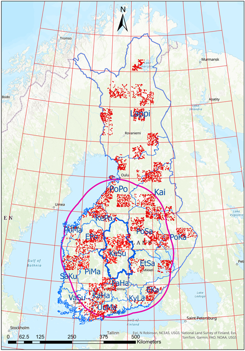
Fig. 1. The forestry districts of Finland (delineated in blue), shown with climate data zones overlaid (red grid). The solid magenta line shows an example of the climate data zones (red grid) within 150 km of the Keski-Suomi (KeSu) forestry district border. The field inventory plot locations shown with red dots. EKa = Etelä-Karjala, EPo = Etelä-Pohjanmaa, EtSa = Etelä-Savo, KaHa = Kanta-Häme, Kai = Kainuu, KePo = Keski-Pohjanmaa, KeSu = Keski-Suomi, KyLa = Kymenlaakso, Lappi = Lappi, PaHa = Päijät-Häme, PiMa = Pirkanmaa, PoKa = Pohjois-Karjala, PoMa = Pohjanmaa, PoPo = Pohjois-Pohjanmaa, PoSa = Pohjois-Savo, SaKu = Satakunta, UuMa = Uusimaa, VaSu = Varsinais-Suomi.
2.2 Field inventory plots
The Finnish Forest Centre (FFC) provided the field inventory plots that we used as the initial state of the sites to be simulated. The data included information on mean tree height, mean tree diameter at breast height, basal area, age, stem volume, stem number, and additional stand information, such as fertility class, development class, dominant tree species and regeneration situation. Site fertility was classified using the Finnish national system based on forest ground vegetation (Cajander 1913; Rantala et al. 2011) using an ordered index (see Supplementary file S1: Table S1). The reference data were acquired during 2019–2021. Table 1 shows the main characteristics of the field plots used in the study.
| Table 1. Statistics of the Finnish Forest Centre field inventory plots used in the study. The total number of plots was 29 619, of which 22 359, 20 537 and 21 181 plots included pine, spruce and broadleaved species, respectively. | |||||
| Variable | Species | Mean | Std | Min | Max |
| Age (year) | Pine | 58.5 | 44.0 | 4 | 385 |
| Spruce | 49.5 | 35.4 | 5 | 300 | |
| Broadleaved | 36.7 | 22.8 | 2 | 180 | |
| Tree height (H) (m) | Pine | 13.1 | 6.5 | 1.3 | 36.5 |
| Spruce | 11.5 | 6.4 | 1.3 | 37.4 | |
| Broadleaved | 11.5 | 6.0 | 1.1 | 37.2 | |
| Tree diameter (D) (cm) | Pine | 17.0 | 8.9 | 0.4 | 58.1 |
| Spruce | 14.4 | 8.6 | 0.3 | 59.8 | |
| Broadleaved | 11.3 | 7.1 | 0.1 | 56.7 | |
| Basal area (BA) (m2 ha–1) | Pine | 11.0 | 8.4 | 0.1 | 54.8 |
| Spruce | 8.0 | 9.9 | 0.1 | 76.3 | |
| Broadleaved | 4.3 | 5.5 | 0.1 | 55.5 | |
2.3 Climate data
Climate data were downloaded from the Copernicus Climate Data Store (Climate Data Store, CDS) using the CDS API client (Copernicus Climate Change Service, Climate Data Store). The CMIP6 climate projections catalogue (CMIP6 climate projections) provides daily and monthly global climate projections data from many experiments, models and time periods computed in the framework of the sixth phase of the Coupled Model Intercomparison Project (CMIP6)(Petrie et al. 2021). The downloaded data included climate model hadgem3_gc31_ll daily data sets for near surface air temperature, near surface specific humidity and precipitation, and the monthly photosynthetically active radiation (PAR) data set for three climate projection experiments (scenarios) following the combined pathways of Shared Socioeconomic Pathway (Shared Socioeconomic Pathway, SSP): ssp1_2_6, ssp2_4_5, and ssp5_8_5 (Gidden et al. 2019). The following variables required by the forest model were retrieved: daily temperature (Tair), precipitation (Precip), vapour pressure deficit (VPD) and monthly PAR. We downloaded the yearly CO2 concentration from CMIP6 Data (Meinshausen et al. 2017) with the ForModLabUHel software available on GitHub (ForModLabUHel). The climate data were acquired for the period 2020–2100.
2.4 Forest growth model
PREBASSO is a process-based, stand-scale forest model developed to simulate the growth, development, and management of forest stands, primarily in boreal and temperate regions. It integrates various ecological processes – including photosynthesis, stand growth, mortality, and regeneration – to predict changes in forest structure and composition over time. In PREBASSO, three interconnected models are combined: PRELES – PREdict Light-use efficiency, Evapotranspiration, and Soil water (Peltoniemi et al. 2015), CROBAS – Tree growth and Crown Base from carbon balance (Mäkelä 1997), and YASSO – Yet Another Simulator of Soil Organic Matter (Liski et al. 2005). PRELES is a light-use efficiency model that predicts gross primary productivity (GPP) and evapotranspiration (ET). The GPP output is utilized by CROBAS to estimate respiration, carbon allocation, and forest growth, based on the pipe model theory. CROBAS also provides inputs such as leaf area index (LAI) to PRELES and litter production data to YASSO. YASSO then simulates soil organic matter dynamics to compute the soil carbon balance (Fig. 2).
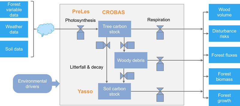
Fig. 2. The biochemical and biophysical modelling system PREBAS.
Forest structural variables (age, diameter at breast-height, DBH (the abbreviation D used later); tree height, H; basal area, BA) are used as input to the model, alongside weather variables and site parameters. The structural variables are provided at the cohort (stratum) level. Additional variables – such as stand volume and tree organ biomasses – are derived from the CROBAS model. Forest development is simulated on an annual time step, whereas photosynthesis and water flux (evapotranspiration) are calculated on a daily time step. The rPrebasso (Mäkelä 1997; Minunno et al. 2016, 2019) software is an R-wrapper that calls the PREBASSO models that have been written in C and Fortran 95 languages. The rPrebasso software package is available on GitHub (rPrebasso, gitHub).
2.5 Test setup and data set construction
We used the rPrebasso software tool to produce yearly forest structure and carbon balance variable predictions for the field inventory plots for 25-year periods. These predictions were used as reference data (or targets) to train the ML models. The time range for the variable prediction was set to 25 years, considered adequate for demonstrating the time series prediction. The predictions were produced for the forest variables: tree height (H), stem diameter (D), basal area (BA), and a subset of carbon balance variables: net primary production (NPP), gross primary production per tree layer (GPP), net ecosystem exchange (NEE) and gross growth (GGR). The variables for different tree species were considered separately, such as the tree height for pine (Hpine), spruce (Hspr), and broadleaved trees (Hbl).
The input variables for rPrebasso tool were 1) the forest variables age, tree height, stem diameter, basal area and species for the initial simulation state, 2) information on the forest site (see Suppl. file S1: Table S2) and 3) the climate data (see paragraph ‘Climate data’ above) for the prediction period.
2.5.1 Training data construction
Neural networks are known for their ability to interpolate modelled functions between training data points, whereas they do not perform well at extrapolating outside data points that they have not seen during the training phase (Bishop 2006; Balestriero et al. 2021). To ensure good generalization in the obtained ML models, we tried to cover the ranges of all realistic input variable combinations and beyond. To get sufficient variation in the ML model training data, the following principles were used in combining data from these two sources (i.e., forest variable + site info data, and climate data):
• The scenario for the selected climate data was selected randomly out of the three options (ssp1_2_6, ssp2_4_5, ssp5_8_5).
• The climate data were obtained in a grid with a spatial resolution of 67–120 km along latitudes (depending on latitude) and 140 km along longitudes. Consequently, the climate data had no variation over areas of size comparable to one forestry district (Fig. 1). To obtain additional variation to the data combinations, the forest variable and site info data were combined with the climate data of the climate data zones within 150 km of the corresponding forestry district border. The climate zone for each site (inventory field plot) was selected randomly from these climate zones. The number of available climate data zones within 150 km of the forestry district borders varied from 17 (KaHa) to 49 (Lappi). The produced climate data and field plot data combinations can still be considered realistic, because the climate data does not change radically between the nearby grid cells.
• The 25-year period of the climate data was selected randomly from within the total range 2020–2100 of the data set.
• The otherwise constant default values of the site info variables (Suppl. file S1: Table S2) were added with random Gaussian noise with σ = 3.0% of the default value.
• The site fertility class was randomly varied with +/– 1 class (within actual min/max limits).
• Considering the relatively big amount of different input data combinations induced by the included climate conditions and the variety of initial forest sites, we decided to exclude the management practices (also available in rPrebasso) and narrowed the study to train the models to predict the undisturbed growth under these different conditions.
The randomized climate data were joined 10 times with each field plot forest variable and the randomized site info data to increase the amount of data for model training (10-fold shuffle). These combined data vectors were provided for rPrebasso as inputs to create the 25-year prediction targets for the ML model. Note that from the point of view of training the ML model there are no correct or incorrect combinations of input data variables, even if some of the produced combinations do not represent any realistic conditions in the forest stands. The produced input- output pairs of data vectors just reflect the non-linear transformation(s) in the target system which we want the ML model to learn (Fig. 3).
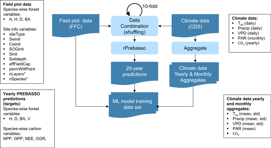
Fig. 3. Training data set construction. The forest variable and site info data from each FFC field plot were combined with the climate data (of random scenario, from random climate zone within 150 km distance from the filed plot’s forestry district border and covering random 25-year period within 2020–2100). The climate data randomized this way were joined 10 times for each field plot (10-fold shuffle). These combined data vectors were provided for rPrebasso as inputs to create the 25-year prediction targets. The climate data were aggregated to contain yearly and monthly averages and standard deviations. The data vector from each field plot were combined with the corresponding 25-year rPrebasso predictions, and aggregated climate data to construct the training data set for the ML models. FFC = Finnish Forest Centre, CDS = Climate Data Store. Forest variables: A = age, H = tree height, D = stem diameter, BA = basal area, V = stem volume; Site info variables: siteType = Site fertility class, Swinit = Initial soil water, Cwinit = Initial crown water, SOGinit = Initial snow on ground, Sinit = Initial temperature acclimation state, Soildepth = Soil depth, effFieldCap = Effective field capacity, permWiltPoint = Permanent wilting point, nLayers = Number of layers*, nSpecies = Number of species*; carbon balance variables: NPP = net primary production, GPP = gross primary production per tree layer, NEE = net ecosystem exchange, GGR = and gross growth; Climate variables: Tair = daily temperature, Precip = precipitation, VPD = vapour pressure deficit, PAR = monthly photosynthetically active radiation, CO2 = yearly CO2 concentration. Species-wise variables were used for the forest and carbon balance variables (e.g. Hpine, Hspr, Hbl; spr = spruce, bl = broadleaved).
*) The variables nLayers and nSpecies used by rPrebasso only, not provided for ML models.
Although rPrebasso uses daily climate data, we computed yearly and monthly aggregates (averages, standard deviations, and cumulative sum of the climate variables PAR, Tair, Precip, and VPD) to be used as inputs to the ML model. This was seen adequate resolution to produce the yearly ML predictions. The field plot data and the climate data aggregates were then combined with the corresponding 25-year rPrebasso predictions to build the ML model training data set. To summarize: each vector of the ML model training data set included thus the forest variables and site info variables from the field plot (initial state of the forest site), the yearly and monthly aggregates of PAR, Tair, Precip, and VPD and the yearly CO2 concentration for a 25-year period (climate data), and the 25-year rPrebasso predictions for the target variables (Fig. 3).
2.5.2 Stratified split of training/validation/test sets
To obtain equal distributions of forest age and species for training, validation and test sets, we composed a stratification variable (As) that combined the ages of different species on a field plot into a single scalar variable, that was then used to sample data vectors to training, validation, and test set by stratified random sampling. We divided As to five strata of equal bin widths and used relative set sizes of 80%, 16% and 4% for the training, validation and test sets, respectively. The stratification variable was a combination of the species-wise ages:
![]()
where Apine, Aspr and Abl are the ages of pine, spruce and broadleaved species in the field plot, respectively; mspr = 300 yrs and mbl = 180 yrs were the maximum ages of spruce and broadleaved trees in the field plot data set, respectively.
According to (Tuominen et al. 2017), the spatial auto-correlation in Finnish forests approaches zero within 200–300 m. Considering this information, we set the minimum distance requirement of the field plots of different data sets (i.e., training, validation or test set) to 250 m and removed all field plots in training and validation sets that did not exceed this threshold.
2.5.3 Handling of missing species data
In a large proportion of the forest plots included in the composed data set there was one or two species (out of three) missing from the field plot. In the data vectors of these plots there were thus empty cells (= vector components), or NULL data, in the missing species forest variables. In general, compensating for missing data is a non-trivial problem in machine learning and different techniques have been proposed (Johnson and Kuhn 2019). The NULL valued species data (vector components) were replaced with actual data sampled randomly from those plots that contained data for this species. This way the distribution of the whole data set did not change significantly. This NULL data replacement method was chosen to ensure that the data used for model training would not induce bias in the model due to distorted input data distributions. The missing (and replaced as explained) species data components of each data vector were identified with dedicated flag variables and excluded from the model performance evaluation.
The resulting data set contained 296 190 data vectors in total, with 29 619 individual forest sites. The training, validation and test sets contained 236 950, 47 390, 11 850 vectors respectively after the stratified split. As all sites did not contain all three species, the test data sets for variables of different species included 7040, 6490 and 6680 vectors for pine, spruce and broadleaved species respectively. To see the effect of training set size on model performance we also created tree height (H) and basal area (BA) models with 32%, 54%, 80% or 100% of the complete data set size. The size of the whole data set was close to 4 gigabytes, when saved as an ASCII text file.
While the rPrebasso takes its inputs as absolute values, all the data for the ML emulator models were normalized to zero mean and unit variance prior to model training and evaluation. The normalization was done for each variable separately, and both for the input data, and the target data.
2.6 The network architectures used in the study
Forecasting forest growth several decades into the future may be seen as an example of time series prediction tasks that may benefit from the ability of deep learning methods to learn complex dependencies between a variety of static and time-dependent inputs and the target time series data. The following neural network architectures were considered relevant for the study.
Recurrent Neural Networks (RNNs) (Rumelhart et al. 1986; Werbos 1990; LeCun et al. 2015) contain recurrent connections, and the output at each time step depends on the previous hidden state and the current input. As the growth of a forest stand follows inherent causality, depending on the status of the previous year, RNNs were seen as a natural choice for modelling the yearly growth.
We included two advanced RNN building block variants, the Gated Recurrent Unit (GRU) (Cho et al. 2014) and Long Short-Term Memory (LSTM) (Hochreiter and Schmidhuber 1997) in our RNN models. The GRU is the simpler of the two, contains fewer trainable parameters and is thus computationally less expensive and faster to train. GRUs also efficiently address the vanishing gradient problem (Hochreiter et al. 2001)
A popular set of architectures used for time series data processing are the sequence-to-sequence (S2S) architectures, also known as encoder-decoder models (Sutskever et al. 2014). These transform one sequence of data into another using an encoder part that processes the input data sequence into a fixed-length context vector that is then provided as input to the decoder part. The decoder then transforms (unfolds) the context vector to the output sequence. The encoder and decoder may contain several stacked recurrent network layers with several time steps, with GRU and LSTM often used as the network building units. The training objective of the encoder-decoder network is to maximise the conditional probability of the output sequence given the input sequence.
The transformer models (Vaswani et al. 2017) also utilize the encoder-decoder architecture. They include attention mechanisms and input positional encoding instead of recurrent connections to resolve long-range dependencies between time series elements (like words or tokens in language processing). Transformers are widely used in natural language processing (NLP) and text generation problems, such as in ChatGPT (Brown et al. 2020), BERT (Devlin et al. 2019) or T5 (Raffel et al. 2023).
A time series of forest growth parameters forms a natural sequence and is a suitable for analysis with RNNs or transformers. Both model types accept multivariate inputs and allow combining the static forest variable and site info features with the temporal climate data.
We tested three network architectures to emulate the Prebasso model. The general architectures of these architectures are presented in Fig. 4.
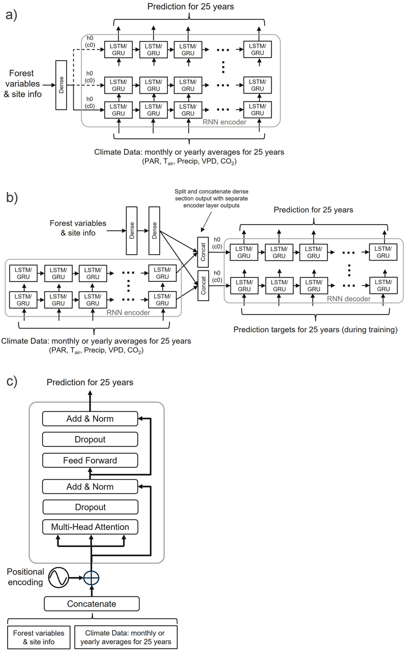
Fig. 4. General overview of the three neural network architectures used in the study: a) RNN encoder with a fully connected input section (FC-RNN), b) RNN encoder-decoder network combined with a fully connected section parallel to the encoder (S2S), and c) Transformer encoder network (TXFORMER). GRU = Gated Recurrent Unit, LSTM = Long short-term memory, PAR = photosynthetically active radiation, TAir = daily temperature, Precip = precipitation, VPD = vapour pressure deficit, CO2 = carbon dioxide, h0 = hidden state vector, c0 = cell state vector, N = number of decoder layers. The reader is suggested to visit the code repository for the detailed implementation of the models.
1) RNN encoder with a fully connected input section (FC-RNN)
This architecture combined the basic Many-to-Many type RNN encoder with a fully connected (dense) input network that took the initial forest site state as input (Fig. 4a). The shape of the of the fully connected section input tensor was (N, Fin), where N = batch size, Fin = number of static variables (= 23). The static variables included the species-wise forest variables for age (Agepine, Agespr, Agebl), tree height (Hpine, Hspr, Hbl), stem diameter (Dpine, Dspr, Dbl), and basal area (BApine, BAspr, BAbl), and eight site information variables of those listed in Suppl. file S1: Table S2. In addition, three binary flag variables indicating the existence of each of the species in the forest stand were included (0 = species does not exist, 1 = species exist).
The output of the fully connected section (shape = (N, Fout)) was fed into the to the encoder hidden state (and cell state with LSTM) initial inputs (h0, c0) and replicated for user selectable number of bottom layers if the encoder contained more than one layer. The dashed arrows in Fig. 4a depict the optional copy of the dense layer outputs to the initial hidden (and cell) state vectors h0, c0 of the RNN encoder. The requirement for the length of the fully connected section output vector was Fout ≤ Hout (Hout = encoder hidden size = the number of features in the hidden state h), and the in case of Fout < Hout, the Hout – Fout components of the hidden (an optionally cell) state initial inputs were initialized to zero (zero-padding).
The input from the dense section to the hidden and cell states of the RNN encoder may be expressed as:
![]()
where ![]() = output vector of the dense section,
= output vector of the dense section, ![]() = zero-padding vector,
= zero-padding vector, ![]() = vector concatenation, l = user selectable number of layers to connect the dense section to (min = 1), nl = number of encoder layers, i = layer index. The batch dimension left out of the formula.
= vector concatenation, l = user selectable number of layers to connect the dense section to (min = 1), nl = number of encoder layers, i = layer index. The batch dimension left out of the formula.
The climate data were fed into the RNN encoder inputs, and the organization and shape of the encoder input tensors were (N, L, Hin), where N = batch size, L = sequence length (= 25), and Hin = input size. The input dimension (3rd dimension) consisted of the yearly or monthly aggregates of the climate variables, and the size of the encoder input tensor was thus (N, L, Hin) = (N × 25 ×12) or (N × 25 × 96) for yearly or monthly climate data respectively.
The shape of the output tensor from the FC_RNN model was (N, L, Hout), where N = batch size, L = sequence length (25), and Hout = output size (number of target variables). The size of the decoder output tensor varied between (N × 25 × 3) and (N × 25 × 12) depending on the number of model output variables (3–12). The number of output variables was always a multiple of three, as we always produced forest or carbon variable models for all three species.
2) RNN encoder-decoder network combined with a fully connected section parallel to the encoder (S2S)
In this architecture, the initial state of the current forest site was provided as input to a fully connected section, that was connected to the RNN decoder part (Fig. 4b). As in the FC_RNN architecture (#1), the shape of the of the fully connected section input tensor was (N, Fin = 23), and the shape of the RNN encoder input, that the climate data were fed into, was (N, L, Hin).
The output of the fully connected section (shape = (N, Fout)) was split into nl (= number of encoder and decoder layers) chunks of equal size along the second dimension, which were then concatenated with the outputs from the different encoder layers to produce the context vectors for the decoder part. These context vectors were then supplied to the decoder hidden (and cell if the RNN unit was LSTM) state inputs. Consequently, the output dimension of the fully connected section was to be an integer multiple of the number of layers in the network. In the trained models we selected the output dimension of the fully connected section to be 24 to allow networks with 1, 2, 3, 4 and 6 layers.
The input from the fully connected section to the hidden and cell states of the RNN decoder may be expressed as:
![]()
where ![]() = the ith split of the dense section output vector, nl = number of decoder layers, and i = layer index.
= the ith split of the dense section output vector, nl = number of decoder layers, and i = layer index. ![]() = context vector from encoder layer i. The batch dimension left out of the formula.
= context vector from encoder layer i. The batch dimension left out of the formula.
With the S2S models we used the teacher forcing (Goodfellow et al. 2016) method and provided the model targets as inputs to the decoder part during model training. The shape of the input and output of the decoder part was (N, L, Hout), where N = batch size, L = sequence length (= 25), and Hout = output size (number of target variables). The size of the decoder output (and input) tensor thus varied between (N × 25 × 3) and (N × 25 × 12), as with the FC_RNN architecture output (#1).
3) Transformer encoder network (TXFORMER)
This network option included the encoder part of the transformer (Vaswani et al. 2017) (Fig. 4c). The initial forest site data was concatenated with the climate data inputs and provided as inputs to the encoder. The forest site data occupied the first one or two elements of the input time series data, and the shape of the encoder input data was then (N, L+1, Hin) or (N, L+2, Hin) depending on whether the climate data included the monthly or yearly aggregates respectively (N = batch size, L = sequence length = 25 years, Hin = encoder input size = 12 or 96). The shape of the output tensor from the transformer encoder model was (N, L, Hout), as with the two other architectures. The transformer encoder input may be expressed as:
where ![]() = transformer encoder input tensor,
= transformer encoder input tensor, ![]() = initial forest site data,
= initial forest site data, ![]() = initial forest site data split in two vectors,
= initial forest site data split in two vectors, ![]() = the yearly climate data vectors,
= the yearly climate data vectors, ![]() = vector concatenation, where the subscript 1 denotes the tensor dimension along which the concatenation is made.
= vector concatenation, where the subscript 1 denotes the tensor dimension along which the concatenation is made.
For the detailed implementation of the models the reader is suggested to visit the code repository in GitHub.
2.7 Custom loss function
Instead of using the standard loss functions available in PyTorch (Paszke et al. 2019), a custom loss function was written to emphasise the bias in the prediction results (Astola et al. 2019; Balazs et al. 2022). The loss function (L) combined the average of the yearly root mean squared error (RMSEave), the average bias (BIASave) and the average mean coefficient of determination (R2ave) computed over all variables predicted by the model being trained:


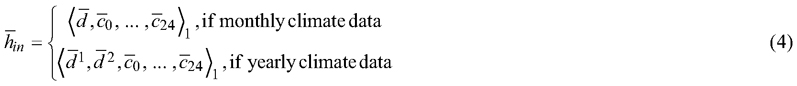
where ![]() , Y is the number of years to predict (sequence length) and K is the number of variables. Definitions of R2, RMSE, and BIAS given in Eq. 7, Eq. 8, and Eq. 10.
, Y is the number of years to predict (sequence length) and K is the number of variables. Definitions of R2, RMSE, and BIAS given in Eq. 7, Eq. 8, and Eq. 10.
2.8 Model performance evaluation
Each test vector included the ML model 25-year predictions and the corresponding rPrebasso target values for the selected variables. Each year of prediction was treated as a separate set of Nt data points (i.e., Nt data points/year, Nt = number of test vectors), for which the RMSE, BIAS and R2 values were computed. Consequently, a set of 25 figures of merit were obtained for each predicted variable. The 25 figures of merit for each predicted variable were then summarised by computing their mean, minimum and maximum values for each variable. As the BIAS may contain both positive and negative values, the mean of the 25 BIAS values may be very close to zero, even if the absolute BIAS values from individual years may significantly differ from zero. We thus included the computation of the mean of the absolute yearly BIAS, denoted as BIAS*, in the summary statistics.
The coefficient of determination R2, absolute and relative root mean square error (RMSE and RMSE%) and absolute and relative bias (BIAS and BIAS%) were defined as:


with ![]() as the target data values (i.e. the rPrebasso predictions) and
as the target data values (i.e. the rPrebasso predictions) and ![]() their mean,
their mean, ![]() as the values predicted by the ML model, and Nt being the total number of samples. All sums are for i = 1,…,Nt.
as the values predicted by the ML model, and Nt being the total number of samples. All sums are for i = 1,…,Nt.
2.9 Optimisation of network structures and hyper-parameters
The best performing network structures and hyper-parameter combinations were optimised for all the different model architectures with a grid search using the validation set loss as the selection criterion. Net primary production (NPP) was used as the target variable to compare the different models. A total of 192 FC-RNN models (111 with GRU, 81 with LSTM), 36 S2S models (18 with GRU, 18 with LSTM), and 51 transformer models were trained with different values of network structure parameters (e.g., hidden dimension or number of layers), and with different values of hyper-parameters (learning rate, batch size and dropout factor) to find well converging models with reasonably good accuracy results.
The FC-RNN obtained the best validation set performance with a network including the LSTM RNN unit, containing four encoder/decoder layers, and with hidden dimension 64. The optimum number of fully connected hidden layers was three. The optimum hyperparameters were learning rate: 0.0005, batch size: 64, dropout factor: 0.2 for both encoder and fully connected section. The optimum structure and hyperparameters, when using the GRU RNN unit were the same, except for the number of fully connected section layers, which was two.
As the differences between the models were extremely small and it turned out that the test set performance results were not always in line with the validation set performance, we reduced the number of varied parameters with S2S model search to reduce the time for the grid search. Fixed values based on FC-RNN experiences were used for S2S model hyper-parameters in the parameter grid search: Number of encoder layers (2), Number of fully connected section hidden layers (1), Learning rate (0.0005), Batch size (64), dropout/encoder (0.2) and dropout/fully connected section (0.2). The found optimum values for encoder hidden dimension, decoder dropout, and for teacher forcing ratio were then 64 (LSTM)/48 (GRU), 0.2, and 0.5 (LSTM)/0.3(GRU) respectively.
With the transformer architecture we found the optimum parameters hidden dimension: 164, number of heads: 16, number of layers: 3, and batch size: 128. With transformer grid search we used the learning rate 0.0005, and dropout factor 0.2.
As the validation set performance was not very sensitive to some of the network structure parameters, we selected values that resulted in a simpler network with fewer trainable parameters (Suppl. file S1: Table S3 – Table S5) for the final models.
2.10 Model implementation and training
The ML model software was written in Python using the PyTorch library with support for GPU computation. Two wrappers were implemented, one for iterating the rPrebasso software to generate the training data, and one for searching for the optimum hyper-parameter values for the different ML models. A separate tool was implemented for training the ML models for the defined variables and for recording the test set performance.
The model software development and the operational tests were carried out on an HP Elitebook laptop computer equipped with Core i7-10610U CPU @ 1.80GHz, and with 24 Gbytes of RAM installed. These test runs included training data typically consisting of 10% to 54% of the whole data set, and they took from a few hours to thirty hours to complete. The optimisation of the hyper-parameters and the model training for the performance evaluation was done in a cloud computing cluster provided for the project by the CSC – IT Center for Science Ltd. (Finland). The model training software was run on a single computing node of CSC’s Puhti supercomputer containing a GPU and four CPUs. The model training on the Puhti supercomputer typically took from two to seven hours to complete (including generation of the data sets for the training function), depending on the amount of training data used (typically 54% or 80% of all training data) and the model complexity. The performance figures of each model were recorded with 80% of the data.
The forest variable models used for the performance results were trained for the nine species-wise variables of tree height, stem diameter, and basal area (Hpine, Hspr, Hbl, Dpine, Dspr, Dbl, BApine, BAspr, BAbl). The models for NPP included the species-wise variables for net primary production (NPPpine, NPPspr, NPPbl) and optionally also the species-wise variables of gross primary production (GPPpine, GPPspr, GPPbl). These models were produced with all the three model architectures. The models for GGR and NEE were produced with FC-RNN model architecture only, as it produced the best results when compared with the forest variable and with NPP and GPP models. These were trained as separate models, with the three species-wise variables as targets in both.
The Table S6 in Suppl. file S1 shows the details of the model architectures and the used hyper-parameters for all the models used for the performance results.
3 Results
3.1 Prediction of Forest Structural and Carbon balance Variables
The forest variable (H, D, BA) models trained using FC-RNN or S2S architecture did not show detectable difference (i.e. larger difference than expected by the inherent randomness in the model training) in terms of test set performance whether using the LSTM or GRU RNN unit as building block. The same applied in using either the yearly or monthly climate data for these models. The best results for the carbon balance variables were obtained with the GRU unit when using the FC-RNN architecture, but with the S2S model there was no detectable difference. Using monthly climate data produced the best carbon balance models, as well as models with transformer architecture.
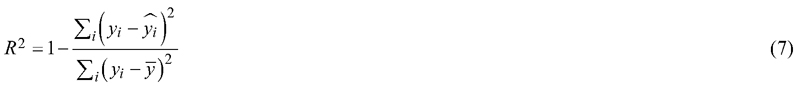
Figs. 5–8 show example prediction curves for tree height (H) and basal area (BA) from two randomly selected test set forest sites. The top row curves in each figure were produced by the FC-RNN model, the middle row by the TXFORMER, and the bottom row curves by the S2S model.
The tree height prediction curves in Fig. 5 indicate relatively small differences between the models. The FC-RNN and S2S model curves progress more smoothly than the TXFORMER prediction in general. The difficulty of the FC-RNN model capturing the progression from the site initial state (year 0) to the first year(s) prediction is clearly visible with variables Hpine and Hbl. This can also be seen for the S2S model variable Hbl.
Fig. 5. Example of 25-year rPrebasso target and ML model prediction curves of tree height (Hpine, Hspr, Hbl) plotted for randomly selected test site (site-ID: 26331). Top row: FC-RNN model, middle row: TXFORMER model, bottom row: S2S model (the model shown in legend). The curves indicate relatively small differences between the models. The FC-RNN and S2S model curves progress more smoothly than the TXFORMER prediction in general. The difficulty of the FC-RNN model capturing the progression from the site initial state (year 0) to the first year(s) prediction is clearly visible with variables Hpine and Hbl. This can also be seen for the S2S model variable Hbl.
The differences between the model types in the basal area prediction curves in Fig. 6 are more distinct than for the tree height curves in Fig. 5. The FC-RNN model seems to best predict the BA progression, although the prediction for broadleaved species (BAbl) contains large offset. The TXORMER curves diverge from the rPrebasso prediction, and the S2S model predictions contain large offset for spruce and broadleaved species.
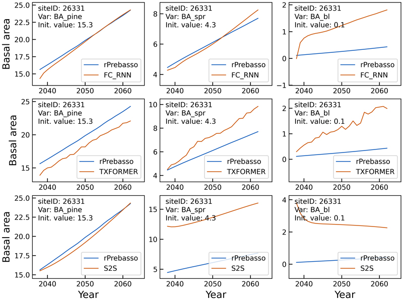
Fig. 6. Example of 25-year rPrebasso target and ML model prediction curves of basal area (BApine, BAspr, BAbl) plotted for randomly selected test site (site-ID: 26331). Top row: FC-RNN model, middle row: TXFORMER model, bottom row: S2S model (the model shown in legend). The differences between the model types are distinct. The FC-RNN model seems to best predict the BA progression, although the prediction for broadleaved species (BAbl) contains large offset.
In the second example of tree height prediction (Fig. 7), the rPrebasso prediction of Hpine saturates after about nine years from the beginning of the prediction period. This behaviour appeared to be difficult to capture by the ML models. The FC-RNN model performs best in replicating the rPrebasso curve, although with large offset. The TXFORMER and S2S models fail to model the saturation. Note that 7.3% of the training data targets (rPrebasso predictions) showed this kind of saturation effect in tree height or stem diameter variables in total. The predictions for Hspr and Hbl are relatively good with all the models on this site.
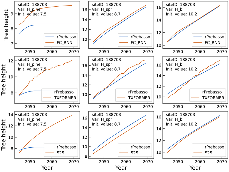
Fig. 7. Example of 25-year rPrebasso target and ML model prediction curves of tree height (Hpine, Hspr, Hbl) plotted for randomly selected test site (site-ID: 188703). Top row: FC-RNN model, middle row: TXFORMER model, bottom row: S2S model (the model shown in legend). The rPrebasso prediction of Hpine saturates after about nine years from the beginning of the prediction period. This behavior appeared to be difficult to capture by the ML models. The FC-RNN model performs best in replicating the rPrebasso curve, although with large offset. TXFORMER and S2S models fail to model the saturation. Note that 7.3% of the training data targets (rPrebasso predictions) showed this kind of saturation effect in tree height or stem diameter variables. The predictions for Hspr and Hbl are relatively good with all the models.
Fig. 8 shows a decline in BApine target (rPrebasso prediction) after about nine years from the beginning of the prediction period, that could be captured by the FC-RNN model only, although with relatively large offset. The TXFORMER and S2S predictions continue increasing with slowly saturating pattern. The TXFORMER predictions contained relatively large variation from year to year, that was not seen in the smother FC-RNN or S2S curves.
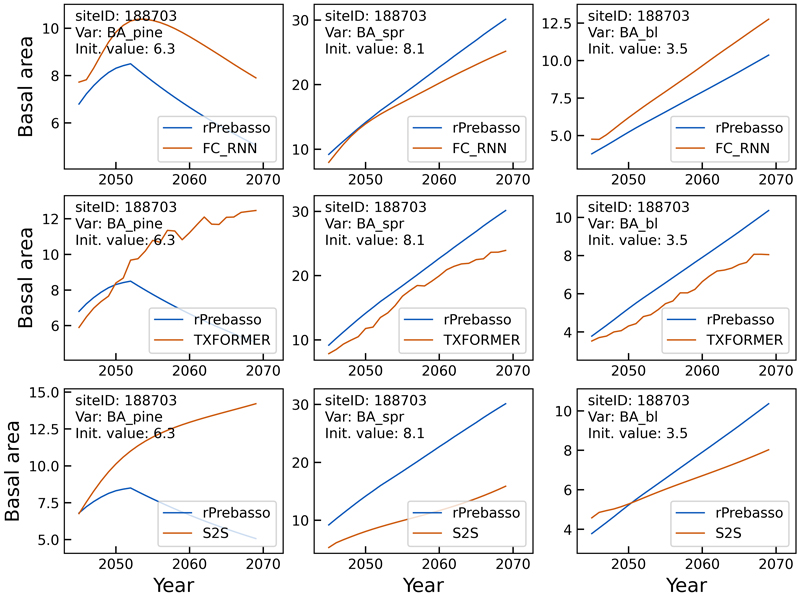
Fig. 8. Example of 25-year rPrebasso target and ML model prediction curves of basal area (BApine, BAspr, BAbl) plotted for randomly selected test site (site-ID: 188703). Top row: FC-RNN model, middle row: TXFORMER model, bottom row: S2S model (the model shown in legend). The decline in BApine target (rPrebasso prediction) after about nine years from the beginning of the prediction period could be captured by the FC-RNN model only, although with relatively large offset.
Table 2 summarizes the best test set performances of the ML models of the three different architectures. The table shows the mean, minimum and maximum of the relative bias and RMS errors of the yearly test set predictions for the forest variables tree height (H), stem diameter (D), basal area (BA), and the carbon balance variable net primary production (NPP). The ‘mean’ bias column shows the mean of the 25-year predictions’ BIAS values, and the ‘mean*’ column shows the mean of the absolute values of the BIAS values (as explained in the section Model performance evaluation).
| Table 2. The mean, minimum and maximum of yearly (25 years) relative bias (BIAS%) and relative root mean squared errors (RMSE%) of the test set predictions computed for tree height (H), tree diameter (D), basal area (BA), and net primary production (NPP) for pine, spruce (spr) and broadleaved (bl) species. Results for model types: FC-RNN, TXFORMER, and S2S compared. LSTM RNN unit in FC_RNN and S2S models used. | |||||||||
| Model type | Variable | Relative bias (BIAS%) | Relative RMS error (RMSE%) | ||||||
| mean | mean* | min | max | mean | min | max | |||
| FC_RNN | Hpine | –0.1 | 0.3 | –0.6 | 0.4 | 6.8 | 6.1 | 8.3 | |
| FC_RNN | Hspr | –0.8 | 0.8 | –1.1 | –0.6 | 6.9 | 6.1 | 8.5 | |
| FC_RNN | Hbl | 0.4 | 0.4 | 0.3 | 0.5 | 5.5 | 5.2 | 6.2 | |
| TXFORMER | Hpine | 0.5 | 0.7 | –1.2 | 1.3 | 7.7 | 6.8 | 9.5 | |
| TXFORMER | Hspr | 0.7 | 0.7 | –0.4 | 1.3 | 8.0 | 6.9 | 10.1 | |
| TXFORMER | Hbl | 0.3 | 0.7 | –1.2 | 1.3 | 6.2 | 5.4 | 7.4 | |
| S2S | Hpine | –0.3 | 0.8 | –1.6 | 1.3 | 11.5 | 9.9 | 14.2 | |
| S2S | Hspr | –1.6 | 1.6 | –2.1 | –0.6 | 11.8 | 10.0 | 14.4 | |
| S2S | Hbl | 0.0 | 0.3 | –1.5 | 0.3 | 11.1 | 10.4 | 14.3 | |
| FC_RNN | Dpine | –0.6 | 0.6 | –0.9 | –0.3 | 6.5 | 5.6 | 8.1 | |
| FC_RNN | Dspr | –0.9 | 0.9 | –1.3 | –0.6 | 7.0 | 6.2 | 8.6 | |
| FC_RNN | Dbl | 0.1 | 0.1 | 0.0 | 0.7 | 6.9 | 6.5 | 8.2 | |
| TXFORMER | Dpine | 0.1 | 0.5 | –1.2 | 1.0 | 8.2 | 6.9 | 10.0 | |
| TXFORMER | Dspr | 0.2 | 0.5 | –1.2 | 0.9 | 10.3 | 9.9 | 11.5 | |
| TXFORMER | Dbl | –1.2 | 1.2 | –3.1 | 0.0 | 8.5 | 8.0 | 9.3 | |
| S2S | Dpine | –0.3 | 0.4 | –1.1 | 0.4 | 14.2 | 12.9 | 16.2 | |
| S2S | Dspr | –0.8 | 0.9 | –1.4 | 0.2 | 14.3 | 12.5 | 16.4 | |
| S2S | Dbl | 1.5 | 1.5 | 0.2 | 1.8 | 14.5 | 13.2 | 18.8 | |
| FC_RNN | BApine | –0.1 | 0.2 | –0.6 | 0.2 | 12.0 | 7.7 | 15.9 | |
| FC_RNN | BAspr | –1.5 | 1.5 | –1.8 | –0.8 | 15.6 | 11.9 | 19.2 | |
| FC_RNN | BAbl | 1.5 | 1.5 | 0.7 | 2.2 | 21.0 | 15.0 | 27.9 | |
| TXFORMER | BApine | –0.7 | 1.5 | –5.0 | 1.5 | 17.6 | 15.2 | 19.7 | |
| TXFORMER | BAspr | 0.8 | 1.0 | –1.4 | 1.8 | 22.1 | 16.4 | 26.5 | |
| TXFORMER | BAbl | –6.4 | 6.4 | –7.4 | –5.0 | 24.7 | 15.6 | 32.5 | |
| S2S | BApine | –0.8 | 1.9 | –3.1 | 3.2 | 45.5 | 41.0 | 54.7 | |
| S2S | BAspr | –10.5 | 10.7 | –17.4 | 2.0 | 63.8 | 61.7 | 67.9 | |
| S2S | BAbl | –21.0 | 21.2 | –34.9 | 2.0 | 86.0 | 82.5 | 99.1 | |
| FC_RNN | NPPpine | 1.2 | 1.3 | –0.1 | 2.4 | 11.6 | 9.9 | 15.5 | |
| FC_RNN | NPPspr | 0.8 | 0.8 | 0.5 | 1.1 | 14.8 | 13.5 | 20.4 | |
| FC_RNN | NPPbl | 1.9 | 1.9 | 0.4 | 3.2 | 22.0 | 20.2 | 28.2 | |
| TXFORMER | NPPpine | –0.7 | 0.9 | –3.6 | 0.7 | 19.9 | 18.5 | 23.6 | |
| TXFORMER | NPPspr | –0.2 | 0.9 | –3.1 | 1.0 | 27.8 | 26.9 | 31.3 | |
| TXFORMER | NPPbl | –2.8 | 2.8 | –4.5 | –1.7 | 30.9 | 28.8 | 32.2 | |
| S2S | NPPpine | 2.6 | 2.6 | –0.4 | 6.3 | 31.2 | 27.4 | 37.9 | |
| S2S | NPPspr | –4.6 | 7.0 | –10.4 | 9.5 | 44.3 | 37.3 | 51.4 | |
| S2S | NPPbl | –17.3 | 17.4 | –26.5 | 1.7 | 64.6 | 59.3 | 88.0 | |
| FC-RNN = recurrent neural network model with fully connected input section; TXFORMER = transformer model. S2S = RNN encoder-decoder model. RNN = Recurrent neural network; LSTM = Long short-term memory. *) The mean of absolute values of BIAS%. | |||||||||
The BIAS% values for the forest variables (Table 2) were well within the specified ±2% limit for the forest variables H and D with all model architectures. The transformer model BIAS% exceeded this level with the variables BAbl and NPPbl, and the S2S architecture BIAS% exceeded this limit with predicted variables BAspr, BAbl, NPPpine, NPPspr, and NPPbl. The species-wise mean relative RMS errors of the FC-RNN model were between 5.5% (Hbl) and 7.0% (Dspr) for tree height (H) and tree diameter (D), and between 12.0% (BApine) and 21.0% (BAbl) for basal area, and between 11.6% (NPPpine) and 22.0% (NPPbl) for net primary production (Table 2). The corresponding species-wise performance figures of the TXFORMER model were slightly higher than with the FC-RNN model and varied between 6.2% (Hbl) and 10.3% (Dspr) for tree height and stem diameter, from 17.6% (BApine) to 24.7% (BAbl) for basal area, and from 19.9% (NPPpine) to 30.9% (NPPbl) for net primary production. The relative RMS values of the S2S models were in general clearly higher than with FC-RNN and TXFORMER models and they varied between 11.1% (Hbl) and 86.0% (BAbl) with the shown variables.
Table 3 shows the same statistics for the RNN encoder model (FC-RNN) for the carbon balance variables gross primary production per tree layer (GPP), gross growth (GGR), and net ecosystem exchange (NEE) for pine, spruce (spr) and broadleaved (bl) species. The mean relative bias (mean*) varied between 0.4% (NEEbl) and 1.9% (GGRpine) and the mean relative RMS error between 10.3% (GPPpine) and 28.0% (GGRbl) with these variables.
| Table 3. The mean, minimum and maximum of yearly (25 years) relative bias (BIAS%) and relative root mean squared errors (RMSE%) of the test set predictions computed for gross primary production per tree layer (GPP), gross growth (GGR), and net ecosystem exchange (NEE) for pine, spruce (spr) and broadleaved (bl) species. GPP model: FC-RNN (GRU). GGR and NEE Models: FC-RNN (LSTM). | ||||||||
| Variable | Relative bias (BIAS%) | Relative RMS error (RMSE%) | ||||||
| mean | mean* | min | max | mean | min | max | ||
| GPPpine | 1.4 | 1.4 | 0.1 | 2.4 | 10.3 | 9.0 | 13.8 | |
| GPPspr | 0.6 | 0.6 | 0.4 | 0.9 | 11.8 | 10.9 | 16.7 | |
| GPPbl | 1.2 | 1.2 | 0.1 | 2.0 | 19.3 | 17.8 | 24.2 | |
| GGRpine | 1.9 | 1.9 | 0.5 | 2.5 | 19.4 | 17.4 | 24.5 | |
| GGRspr | –1.4 | 1.4 | –2.3 | –0.7 | 19.2 | 18.1 | 23.3 | |
| GGRbl | 0.2 | 0.6 | –0.6 | 1.6 | 28.0 | 25.4 | 31.3 | |
| NEEpine | 0.8 | 0.8 | 0.4 | 1.7 | 13.2 | 11.0 | 17.4 | |
| NEEspr | 1.3 | 1.3 | 0.5 | 1.9 | 17.4 | 15.8 | 20.6 | |
| NEEbl | 0.4 | 0.4 | –0.2 | 1.4 | 25.4 | 23.7 | 27.3 | |
| FC-RNN = recurrent neural network model with fully connected input section; RNN = Recurrent neural network; LSTM = Long short-term memory; GRU = Gated recurrent unit. *) The mean of absolute values of BIAS%. | ||||||||
Figs. 9 and 10 show the scatterplots of H and BA test set predictions against rPrebasso estimates (target) for years 5, 12 and 25. The model architecture was FC-RNN with LSTM units. Although the errors of the variable predictions tend to increase towards the end of the 25-year period, the BIAS% remains at moderately low levels. For additional examples, see Suppl. file S1: Figures S1–S4.
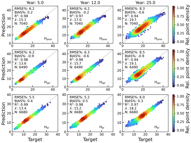
Fig. 9. Scatterplots of test set tree height predictions for pine (Hpine), spruce (Hspr) and broadleaved (Hbl) species against rPrebasso estimates (target) for years 5, 12 and 25. Model = FC-RNN (LSTM). RMSE% = relative RMS-error, BIAS% = relative bias, R2 = coefficient of determination, ![]() = the average of the target values, N = number of samples. The colour shows the relative density of the graph points. FC-RNN = RNN encoder model with a fully connected input section; LSTM = Long short-term memory. RNN = Recurrent neural network.
= the average of the target values, N = number of samples. The colour shows the relative density of the graph points. FC-RNN = RNN encoder model with a fully connected input section; LSTM = Long short-term memory. RNN = Recurrent neural network.
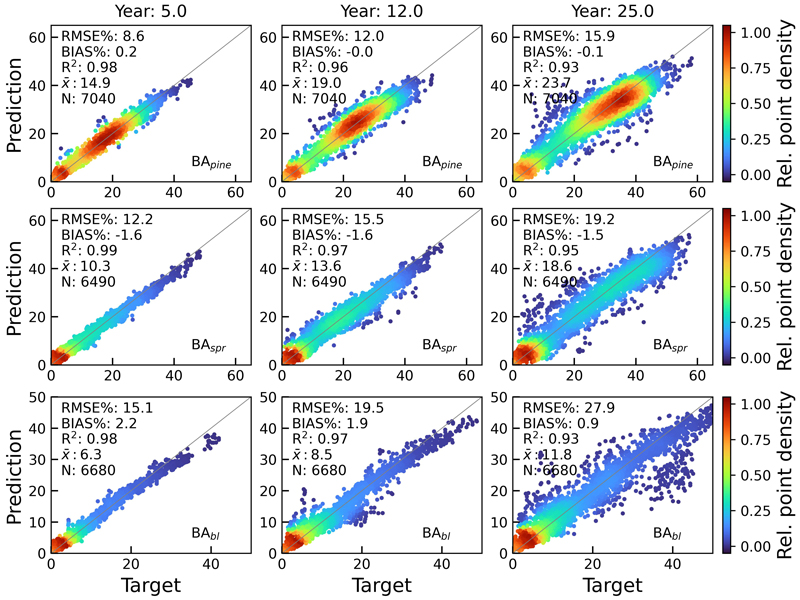
Fig. 10. Scatterplots of test set basal area predictions for pine (BApine), spruce (BAspr) and broadleaved (BAbl) species against rPrebasso estimates (target) for years 5, 12 and 25. Model = FC-RNN (LSTM). RMSE% = relative RMS-error, BIAS% = relative bias, R2 = coefficient of determination, ![]() = the average of the target values, N = number of samples. The colour shows the relative density of the graph points. FC-RNN = RNN encoder model with a fully connected input section; LSTM = Long short-term memory. RNN = Recurrent neural network.
= the average of the target values, N = number of samples. The colour shows the relative density of the graph points. FC-RNN = RNN encoder model with a fully connected input section; LSTM = Long short-term memory. RNN = Recurrent neural network.
Figs. 11 and 12 show the boxplots of the residuals of tree height and basal area predictions of FC-RNN (LSTM) model respectively. An increase in the prediction variance towards the end of the prediction period is clearly visible, but the mean of the residuals remains quite stable and close to zero, reflecting low bias. With the shown variables there was a decrease in variance at the beginning of the 25-year period with the variance reaching its minimum within years 3–5. The reason for the larger variance in the first years reflects the difficulty of the FC-RNN model to model the progression from the site initial state (year 0) to the first year(s) prediction seen in the prediction curves (Figs. 5–8). This was not visible in the residual boxplots of the transformer model (see Suppl. file S1: Figures S5–S6).
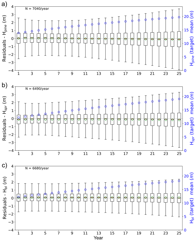
Fig. 11. Boxplots of test set yearly residual errors for the tree height of a) pine (Hpine), b) spruce (Hspr) and c) broadleaved (Hbl) species. Model: FC-RNN (LSTM). Green diamond = mean, red line = median. Right hand scale: the yearly mean of the target variable (plotted with blue circles). FC-RNN = RNN encoder model with a fully connected input section; LSTM = Long short-term memory. RNN = Recurrent neural network.
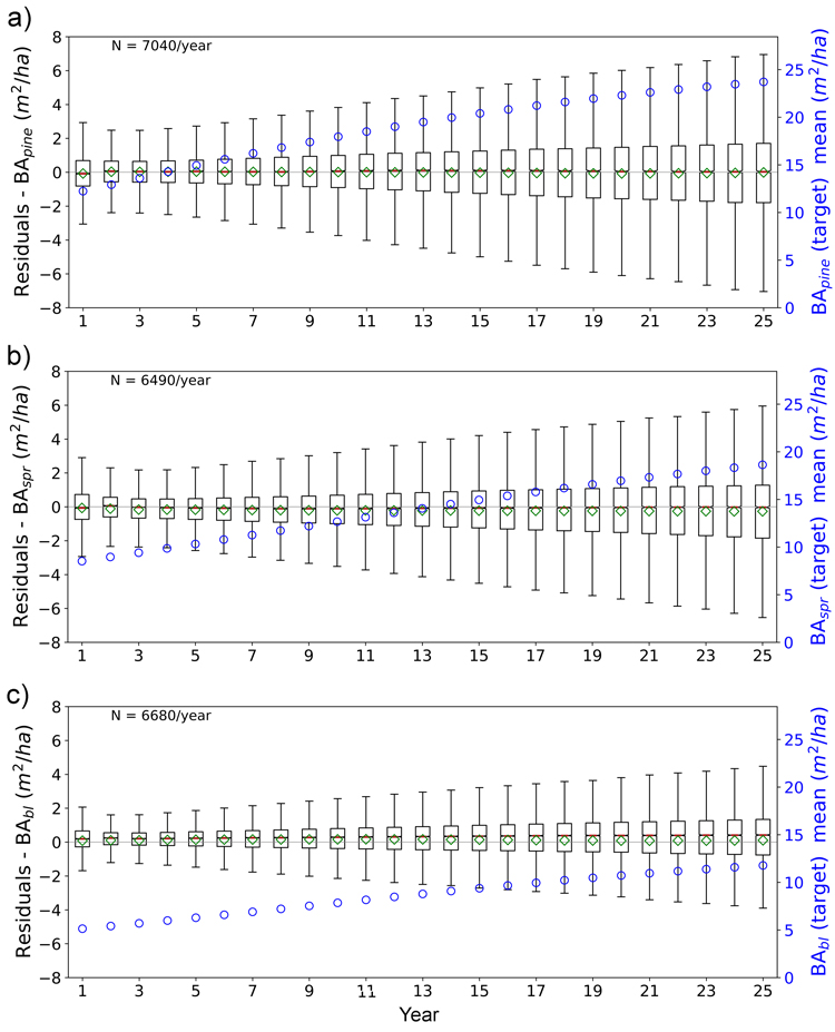
Fig. 12. Boxplots of test set yearly residual errors for the basal area of a) pine (BApine), b) spruce (BAspr) and c) broadleaved (BAbl) species. Model: FC-RNN (LSTM). Green diamond = mean, red line = median. Right hand scale: the yearly mean of the target variable (plotted with blue circles). FC-RNN = RNN encoder model with a fully connected input section; LSTM = Long short-term memory. RNN = Recurrent neural network.
The plots in Figs. 13–16 show the test set BIAS% and RMSE% for year 25 for tree height (H) and basal area (BA) for each site type (quantified as fertility class), showing the effect of the training data distribution. Approx. 83% of the training data belonged to fertility classes 2–4 which is reflected in the generally smaller error figures for these classes. As a rule, the predictions showed the largest overestimates for the poorest sites (5 and 6) and the largest underestimates for the richest sites (1) (Fig. 13 and 15). As an exception to this, Hpine and BApine were also overestimated for the richest sites.
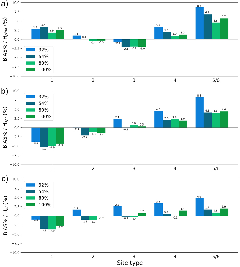
Fig. 13. The test set relative bias (BIAS%) for year 25 plotted per site type for the tree height of a) pine (Hpine), b) spruce (Hspr) and c) broadleaved (Hbl) species. The bars of different colours represent models trained with 32%, 54%, 80% or 100% of the training data set. The fertility classes 5 and 6 were treated as a single class by rPrebasso. Model FC-RNN (LSTM). FC-RNN = RNN encoder model with a fully connected input section; LSTM = Long short-term memory. RNN = Recurrent neural network.
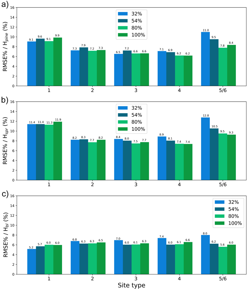
Fig. 14. The test set relative RMS error (RMSE%) for year 25 plotted per site type for the tree height of a) pine (Hpine), b) spruce (Hspr) and c) broadleaved (Hbl) species. The bars of different colours represent models trained with 32%, 54%, 80% or 100% of the training data set. The fertility classes 5 and 6 were treated as a single class by rPrebasso. Model FC-RNN (LSTM). FC-RNN = RNN encoder model with a fully connected input section; LSTM = Long short-term memory. RNN = Recurrent neural network.
To see the effect of the size of the training data set on model performance, we plotted the errors for the models trained with 32%, 54%, 80% or 100% of the training data set with bars of different colour in Figs. 13–16. In most cases the lowest relative RMS error (per fertility class) was achieved with the model trained with 80% or 100% of the training data (Fig. 14 and 16). This was also true for the relative BIAS, although there was more variation between the fertility classes (Fig. 13 and 15). The clearest decreasing trend of increasing training set size can be seen in the basal area RMSE%. It is noteworthy that using 100% of the training data did not bring any significant improvement to the results when compared to using 80%. For tree height and basal area relative errors plotted for age categories, see Suppl. file S1: Figures S7–S10.
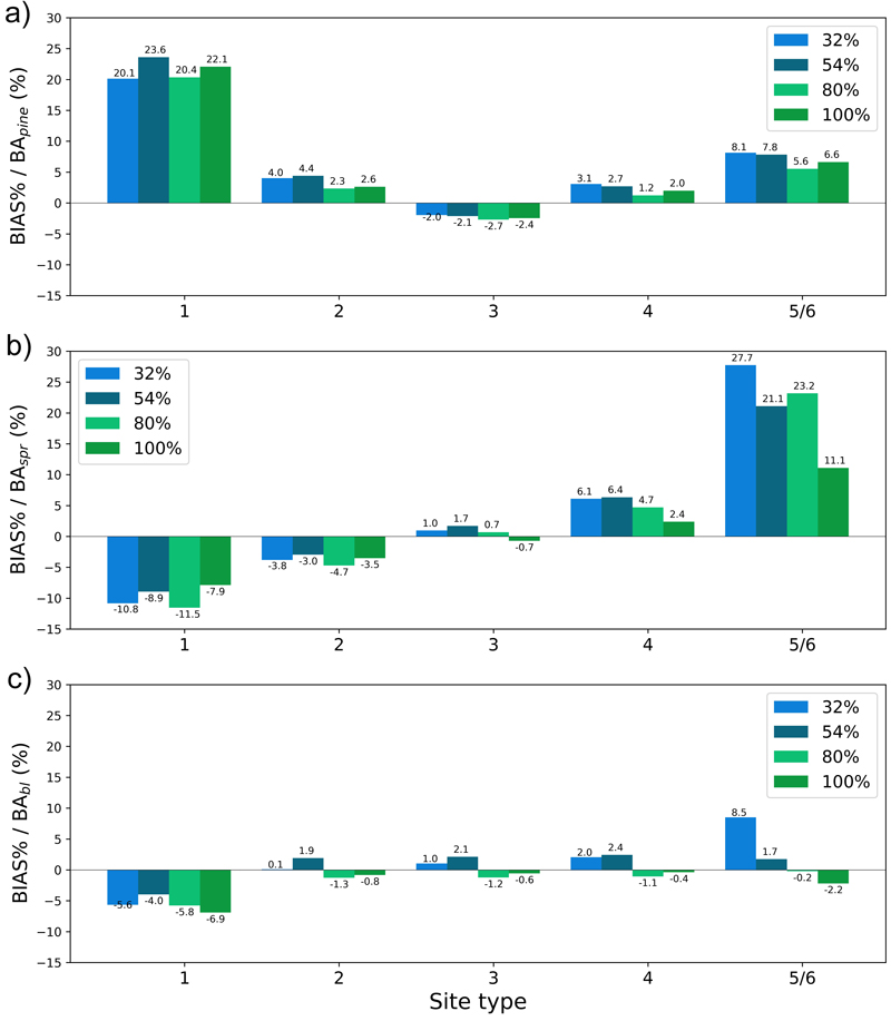
Fig. 15. The test set relative bias (BIAS%) for year 25 plotted per site type category for the basal area of a) pine (BApine), b) spruce (BAspr) and c) broadleaved (BAbl) species. The bars of different colours represent models trained with 32%, 54%, 80% or 100% of the training data set. The fertility classes 5 and 6 were treated as a single class by rPrebasso. Model FC-RNN (LSTM). FC-RNN = RNN encoder model with a fully connected input section; LSTM = Long short-term memory. RNN = Recurrent neural network.
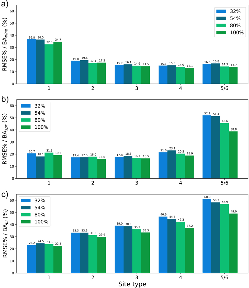
Fig. 16. The test set relative RMS error (RMSE%) for year 25 plotted per site type category for the basal area of a) pine (BApine), b) spruce (BAspr) and c) broadleaved (BAbl) species. The bars of different colours represent models trained with 32%, 54%, 80% or 100% of the training data set. The fertility classes 5 and 6 were treated as a single class by rPrebasso. Model FC-RNN (LSTM). FC-RNN = RNN encoder model with a fully connected input section; LSTM = Long short-term memory. RNN = Recurrent neural network.
To verify the coherence of the produced forest variable predictions we computed the correlations (Pearson-correlation) between the 25-year predictions of tree height (H) and stem diameter (D), as we considered that the most important correlation between the forest structural variables was the relationship between these two variables. The correlations were computed for the species wise variables, and we included the corresponding results of the rPrebasso predictions for comparison. Table 4 summarizes the results for the three model architectures. All the different model types preserved the tree height and stem diameter coherence, especially the TXFORMER and S2S models.
| Table 4. The mean, minimum, maximum, and standard deviation of the correlation between the species-wise tree height (H) and stem diameter (D) predictions of test data set. The results of rPrebasso predictions indicated by the suffix ‘PR’, and the results of the machine learning models by the suffix ‘ML’. Results of the three model types FC-RNN (LSTM), TXFORMER, and S2S (LSTM) compared. | ||||||||||
| Model | Species | mean_PR | min_PR | max_PR | std_PR | mean_ML | min_ML | max_ML | std_ML | N |
| FC_RNN | pine | 0.999 | 0.993 | 1.000 | 0.001 | 0.993 | –0.013 | 1.000 | 0.032 | 7040 |
| FC_RNN | spr | 0.989 | –1.000 | 1.000 | 0.127 | 0.994 | –0.696 | 1.000 | 0.049 | 6490 |
| FC_RNN | bl | 0.999 | 0.400 | 1.000 | 0.015 | 0.995 | –0.407 | 1.000 | 0.027 | 6680 |
| TXFORMER | pine | 0.999 | 0.993 | 1.000 | 0.001 | 0.996 | 0.565 | 1.000 | 0.017 | 7040 |
| TXFORMER | spr | 0.989 | –1.000 | 1.000 | 0.127 | 0.997 | 0.901 | 1.000 | 0.004 | 6490 |
| TXFORMER | bl | 0.999 | 0.400 | 1.000 | 0.015 | 0.997 | 0.440 | 1.000 | 0.014 | 6680 |
| S2S | pine | 0.999 | 0.993 | 1.000 | 0.001 | 0.996 | 0.889 | 1.000 | 0.005 | 7040 |
| S2S | spr | 0.989 | –1.000 | 1.000 | 0.127 | 0.997 | 0.959 | 1.000 | 0.003 | 6490 |
| S2S | bl | 0.999 | 0.400 | 1.000 | 0.015 | 0.994 | 0.585 | 1.000 | 0.029 | 6680 |
4 Discussion
We compared the performance of three different neural network architectures in predicting forest growth parameters for 25 years. For most of the selected variables the test set mean relative BIAS was within the required ±2.0% limit with the test setup used, and the mean relative RMS error varied between 5.1% and 26.1% with the best model architecture. When investigated by site type, the BIAS% and RMSE% values were higher. This was expected as all model predictions average the phenomenon modelled. This was clearly seen in overestimates of height and basal area on poor sites and in underestimates on the richest sites. The architecture with the combined fully connected section and an RNN encoder module (FC-RNN model) produced the best results, while the somewhat more complex RNN architecture with both encoder and decoder parts and with a larger number of trainable parameters (S2S model) produced clearly higher error levels. The models with transformer architecture (TXFORMER) did not achieve as good results as the FC-RNN models, albeit the differences in the case of the best models were relatively small. This was not surprising as we used only the very basic (vanilla) transformer encoder architecture. The usage of more advanced variants of transformers, like with relative positional self-attention (Shaw et al. 2018), or to use Learnable Positional Encoding (Zerveas et al. 2021) could have improved the results. One reason for this might also be that we did not use the whole transformer architecture in our models, just the encoder part. Verification of this and the usage of more advanced transformer methods for the current application are subjected to a possible future study.
We did not see very clear difference in using the LSTM or GRU RNN unit in the recurrent network models, although the best validation set errors were obtained with LSTM in the model parameter grid search (with small margin to GRU models). The LSTM unit seemed to give some advantage with the carbon variables net ecosystem exchange (NEE) and gross growth (GGR), but as we did not perform any systematic tests with these variables, the question remains open. Using yearly climate data in the ML model inputs were found to be adequate for training the forest variable models. Instead, the models for the carbon balance variables required the more detailed monthly data. This reflects the more demanding nature of these variables and consequently the need of more detailed input data.
In general, the errors of the forest structural variables were smaller than the errors of the carbon flux variables. This was expected as the carbon flux and growth variables reflect annual variations and depend on weather inputs and forest state. The forest structural variables, such as stem diameter, tree height and basal area, are cumulative over time and thus generally produce lower errors. The basal area variable has higher error compared to stem diameter and tree height as it depends more on ecosystem dynamics such as mortality which might be more difficult for the emulator to capture. As we modelled the forest variables together, optimizing by punishing deviation of a forest state vector from the prediction of a process-based growth model the mutual coherence of the variables was good. The used modelling scheme included a strong and explicit requirement of physicality in the emulation process, in contrast to the case when building individual models for each variable.
The training data set in our study consisted of 296 190 data vectors. For complex deep learning models, this is a rather small sample. Therefore, an interesting question would be whether the model’s performance could be further improved with a training data set larger, e.g., by a factor of ten. In our tests the effect of the training set size on the model performance was not very clear, although the best results were generally obtained with the two largest training sets. The inherent randomness in the model training process brings uncertainty to the performance metrics of the models, and more comprehensive tests should be run to see the significance of the training set size.
One issue with ML models is that they sometimes poorly learn the cases that represent small minorities in the data set (Sangalli et al. 2022). This behaviour was also seen in our test setup when comparing results between the smallest and largest strata: the errors for the rare fertility classes (1, 5 and 6) were clearly higher than for the most common classes (2–4). The same effect was seen when plotting the errors against age categories. Special attention must thus be paid when generating the training data set to cover the intended use cases of the model adequately. Consequently, instead of solely concentrating on increasing the size of the training data set to improve model performance, it is crucial to investigate the training data distributions in detail, and the characteristics of the cases (i.e., forest sites) that produce the largest errors.
In empirical data, the most under-represented cases are old forests on rich soils, as they are mostly harvested before they get old, leading to most old forests growing on poor soils. This is an important source of bias. Moreover, one very under-represented case is untreated and over-stocked stands. There was no empirical data on them in our data set as most forests in Finland are managed. Consequently, it is highly likely that the development of such forests is largely over-estimated (Hynynen et al. 2014).
Efficient usage of ML models depends on data availability and quality: high-quality, large-scale data sets are essential for training machine learning models. In our case the production of large data sets will not be a problem, but the data quality may become an issue: even though neural network models are known to filter random noise present in the training data set to some extent (Bishop 2006), emulator models are prone to learn the systematic errors present in the underlying physical model. Therefore, it is important that the ML model does not introduce further bias into the predictions. On the other hand, the ML model may be configured to be refined with empirical forest data to reduce these errors, if this kind of data are available.
An alternative approach to using an emulator with training data obtained from a forest simulator (such as Prebasso) is to train a data driven machine learning forest growth simulator using forest inventory data from fixed locations (Magalhaes et al. 2022; Jevšenak et al. 2023). This would avoid adding noise from the intermediate (analytical) model producing simulated training data. However, an accurate description of the causal relationships requires large plots and a long time series. Data accuracy, including a lack of bias, is very important especially in long-term predictions. Thus, data from standard inventory plots covering a short period are not good data sources for growth modelling (Hynynen et al. 2002).
As was seen in the prediction curve plots, the FC-RNN and S2S models’ ability to capture the progression from the site initial status to the first year(s) prediction was not perfect. This implies that there is a need to modify the used architectures or the model training setup for the ML model to deduce this dependency. One solution might be to add a ‘year zero output’ to the models with the forest site initial site state as target for the model to learn the identity transformation and then possibly the causal dependencies in the data more accurately.
The results shown here demonstrate the performance of only a very basic set of architectural concepts to achieve the study objectives. Recent advances in deep learning offer a wide variety of techniques to improve the accuracy of time series prediction, including combining attention mechanisms with RNN encoder-decoder networks (Niu et al. 2021), applying advanced signal processing techniques with recurrent networks (Bi et al. 2024) or using residual connections (Wu et al. 2016). We recommend further investigation of these techniques when ML emulators are applied in practice in the future.
Our study shows that emulating the operation of analytical forest growth models is feasible using state-of-the-art machine learning methods. In the future, the errors of the process-based forest growth model should be analysed together with the emulation errors using measured forest and meteorological time series to achieve the best possible parameterisation and quantify the uncertainty of the whole modelling process.
Declaration of openness of research materials, data, and code
• Access to research code and their metadata: https://github.com/vttresearch/forest_growth_model_emulator.git.
• Access to research data sets and their metadata: https://doi.org/10.5281/zenodo.18186624.
• The CMIP6 climate projection data: https://cds.climate.copernicus.eu/datasets/projections-cmip6?tab=overview.
• The CO2 concentrations for climate scenarios ssp-1.2.6, ssp-2.4.5, and ssp-5.8.5: https://github.com/ForModLabUHel/utilStuff/tree/master/CopernicusData.
• The forest inventory data: https://avoin.metsakeskus.fi/aineistot/Inventointikoealat/Maakunta/.
Authors’ contributions
Conceptualization of the research and design of the work: H. Astola, M. Mõttus, F. Minunno, A. Kangas; The data acquisition, data analysis, and producing results: H. Astola; Interpretation of data and results: H. Astola, A. Kangas, F. Minunno, M. Mõttus; Scientific writing of the work – original draft: H. Astola, M. Mõttus; Manuscript critical revision and incremental writing: H. Astola, A. Kangas, F. Minunno, M. Mõttus. All authors have read and agreed to the manuscript version to be published.
Acknowledgements
We acknowledge the World Climate Research Programme, which, through its Working Group on Coupled Modelling, coordinated and promoted CMIP6. We thank the climate modelling groups for producing and making available their model output, the Earth System Grid Federation (ESGF) for archiving the data and providing access, and the multiple funding agencies who support CMIP6 and ESGF.
The field reference data for the PREBASSO model were provided by the Finnish Forest Centre. The authors wish to acknowledge CSC – IT Center for Science, Finland, for computational resources.
Funding
This work was funded by the Research Council of Finland under grant number 348035 (project ARTISDIG). It also received funding from the European Union’s NextGenerationEU instrument and the Horizon Europe TerraDT project (number 101187992).
References
Astola H, Häme T, Sirro L, Molinier M, Kilpi J (2019) Comparison of Sentinel-2 and Landsat 8 imagery for forest variable prediction in boreal region. Remote Sens Environ 223: 257–273. https://doi.org/10.1016/j.rse.2019.01.019.
Balazs A, Liski E, Tuominen S, Kangas A (2022) Comparison of neural networks and k-nearest neighbors methods in forest stand variable estimation using airborne laser data. ISPRS Open J Photogramm Remote Sens 4, article id 100012. https://doi.org/10.1016/j.ophoto.2022.100012.
Balestriero R, Pesenti J, LeCun Y(2021) Learning in high dimension always amounts to extrapolation. arXiv, article id 2110.09485. https://doi.org/10.48550/arXiv.2110.09485.
Barredo Arrieta A, Díaz-Rodríguez N, Del Ser J, Bennetot A, Tabik S, Barbado A, Garcia S, Gil-Lopez S, Molina D, Benjamins R, Chatila R, Herrera F (2020) Explainable Artificial Intelligence (XAI): concepts, taxonomies, opportunities and challenges toward responsible AI. Inf Fusion 58: 82–115. https://doi.org/10.1016/j.inffus.2019.12.012.
Bauer P, Stevens B, Hazeleger W (2021) A digital twin of Earth for the green transition. Nat Clim Chang 11: 80–83. https://doi.org/10.1038/s41558-021-00986-y.
Bengio Y (2012) Deep learning of representations for unsupervised and transfer learning. In: Guyon I, Dror G, Lemaire V, Taylor G, Silver D (eds) Proceedings of ICML Workshop on Unsupervised and Transfer Learning. PMLR, Bellevue, Washington, pp 17–37.
Bi J, Chen Z, Yuan H, Zhang J (2024) Accurate water quality prediction with attention-based bidirectional LSTM and encoder–decoder. Expert Syst Appl 238, article id 121807. https://doi.org/10.1016/j.eswa.2023.121807.
Bishop CM (2006) Pattern recognition and machine learning. Springer. ISBN 978-0-387-31073-2.
Blanco JA, Lo Y-H (2023) Latest trends in modelling forest ecosystems: new approaches or just new methods? Curr For Rep 9: 219–229. https://doi.org/10.1007/s40725-023-00189-y.
Brown TB, Mann B, Ryder N, Subbiah M, Kaplan J, Dhariwal P, Neelakantan A, Shyam P, Sastry G, Askell A, Agarwal S, Herbert-Voss A, Krueger G, Henighan T, Child R, Ramesh A, Ziegler DM, Wu J, Winter C, Hesse C, Chen M, Sigler E, Litwin M, Gray S, Chess B, Clark J, Berner C, McCandlish S, Radford A, Sutskever I, Amodei D (2020) Language models are few-shot learners. In: Larochelle H, Ranzato M, Hadsell R, Balcan MF, Lin H (eds) Advances in Neural Information Processing Systems 33 (NeurIPS 2020). ISBN 9781713829546.
Cajander AK (1913) Ueber Waldtypen. [About forest site types]. Acta For Fenn 1. https://doi.org/10.14214/aff.7526.
Cho K, van Merrienboer B, Gulcehre C, Bahdanau D, Bougares F, Schwenk H, Bengio Y (2014) Learning phrase representations using RNN Encoder-Decoder for statistical machine translation. In: Moschitti A, Pang B, Daelemans W (eds) Proceedings of the 2014 Conference on Empirical Methods in Natural Language Processing (EMNLP), Doha, Qatar. Association for Computational Linguistics, pp 1724–1734. https://doi.org/10.3115/v1/D14-1179.
Dagon K, Sanderson BM, Fisher RA, Lawrence DM (2020) A machine learning approach to emulation and biophysical parameter estimation with the Community Land Model, version 5. Adv Stat Climatol Meteorol Oceanogr 6: 223–244. https://doi.org/10.5194/ascmo-6-223-2020.
Devlin J, Chang M-W, Lee K, Toutanova K (2019) BERT: pre-training of deep bidirectional transformers for language understanding. In: Burstein J, Doran C, Solorio T (eds) Proceedings of NAACL-HLT 2019, pp 4171–4186. https://doi.org/10.18653/v1/N19-1423.
Fletcher CG, McNally W, Virgin JG, King F (2022) Toward efficient calibration of higher‐resolution earth system models. J Adv Model Earth Syst 14, article id e2021MS002836. https://doi.org/10.1029/2021MS002836.
Foley JA, Prentice IC, Ramankutty N, Levis S, Pollard D, Sitch S, Haxeltine A (1996) An integrated biosphere model of land surface processes, terrestrial carbon balance, and vegetation dynamics. Global Biogeochem Cycles 10: 603–628. https://doi.org/10.1029/96GB02692.
Gidden MJ, Riahi K, Smith SJ, Fujimori S, Luderer G, Kriegler E, van Vuuren DP, van den Berg M, Feng L, Klein D, Calvin K, Doelman JC, Frank S, Fricko O, Harmsen M, Hasegawa T, Havlik P, Hilaire J, Hoesly R, Horing J, Popp A, Stehfest E, Takahashi K (2019) Global emissions pathways under different socioeconomic scenarios for use in CMIP6: a dataset of harmonized emissions trajectories through the end of the century. Geosci Model Dev 12: 1443–1475. https://doi.org/10.5194/gmd-12-1443-2019.
Goodfellow I, Bengio Y, Courville A (2016) Deep learning. MIT Press.
Haara A, Leskinen P (2009) The assessment of the uncertainty of updated stand-level inventory data. Silva Fenn 43: 87–112. https://doi.org/10.14214/sf.219.
Hochreiter S, Schmidhuber J (1997) Long short-term memory. Neural Comput 9: 1735–1780. https://doi.org/10.1162/neco.1997.9.8.1735.
Hochreiter S, Bengio Y, Frasconi P, Schmidhuber J (2001) Gradient flow in recurrent nets: the difficulty of learning long-term dependencies. In: Kremer SC, Kolen JF (eds) A field guide to dynamical recurrent neural networks. IEEE Press. ISBN 978-0-780-35369-5.
Hoffmann J, Bauer P, Sandu I, Wedi N, Geenen T, Thiemert D (2023) Destination Earth – a digital twin in support of climate services. Clim Serv 30, article id 100394. https://doi.org/10.1016/j.cliser.2023.100394.
Hynynen J, Ojansuu R, Hökkä H, Siipilehto J, Salminen H, Haapala P (2002) Models for predicting stand development in MELA system. Finnish Forest Research Institute Research Papers 835. https://urn.fi/URN:ISBN:951-40-1815-X.
Hynynen J, Salminen H, Ahtikoski A, Huuskonen S, Ojansuu R, Siipilehto J, Lehtonen M, Rummukainen A, Kojola S, Eerikäinen K (2014) Scenario analysis for the biomass supply potential and the future development of Finnish forest resources. Working Papers of the Finnish Forest Research Institute 302. https://urn.fi/URN:ISBN:978-951-40-2487-0.
Jevšenak J, Arnič D, Krajnc L, Skudnik M (2023) Machine Learning Forest Simulator (MLFS): R package for data-driven assessment of the future state of forests. Ecol Inform 75, article id 102115. https://doi.org/10.1016/j.ecoinf.2023.102115.
Johnson K, Kuhn M (2019) Feature engineering and selection: a practical approach for predictive models. Chapman and Hall/CRC. ISBN 9781032090856.
Kangas A, Pitkänen TP, Mehtätalo L, Heikkinen J (2023) Mixed linear and non-linear tree volume models with regional parameters to main tree species in Finland. Forestry 96: 188–206. https://doi.org/10.1093/forestry/cpac038.
Kangas AS (1997) On the prediction bias and variance in long-term growth projections. For Ecol Manage 96: 207–216. https://doi.org/10.1016/S0378-1127(97)00056-X.
Kangas AS (1999) Methods for assessing uncertainty of growth and yield predictions. Can J For Res 29: 1357–1364. https://doi.org/10.1139/x99-100.
Kolehmainen I (2001) Hyvän metsänhoidon suositukset. Metsätalouden kehittämiskeskus Tapio. ISBN 952-9891-76-8.
Köppen W (2011) The thermal zones of the Earth according to the duration of hot, moderate and cold periods and to the impact of heat on the organic world. Meteorologische Zeitschrift 20: 351–360. https://doi.org/10.1127/0941-2948/2011/105.
Lecun Y, Bengio Y, Hinton G (2015) Deep learning. Nature 521: 436–444. https://doi.org/10.1038/nature14539.
Liski J, Palosuo T, Peltoniemi M, Sievänen R (2005) Carbon and decomposition model Yasso for forest soils. Ecol Modell 189: 168–182. https://doi.org/10.1016/j.ecolmodel.2005.03.005.
Magalhaes JG de S, Polinko AP, Amoroso MM, Kohli GS, Larson BC (2022) The Predicting Tree Growth app: an algorithmic approach to modelling individual tree growth. Ecol Modell 467, article id 109932. https://doi.org/10.1016/j.ecolmodel.2022.109932.
Mäkelä A (1997) A carbon balance model of growth and self-pruning in trees based on structural relationships. For Sci 43: 7–24. https://doi.org/10.1093/forestscience/43.1.7.
Mehtätalo L, Lappi J (2020) Biometry for forestry and environmental data: with examples in R. Chapman and Hall/CRC, New York. https://doi.org/10.1201/9780429173462.
Meinshausen M, Vogel E, Nauels A, Lorbacher K, Meinshausen N, Etheridge DM, Fraser PJ, Montzka SA, Rayner PJ, Trudinger CM, Krummel PB, Beyerle U, Canadell JG, Daniel JS, Enting IG, Law RM, Lunder CR, O’Doherty S, Prinn RG, Reimann S, Rubino M, Velders GJM, Vollmer MK, Wang RHJ, Weiss R (2017) Historical greenhouse gas concentrations for climate modelling (CMIP6). Geosci Model Dev 10: 2057–2116. https://doi.org/10.5194/gmd-10-2057-2017.
Minunno F, Peltoniemi M, Launiainen S, Aurela M, Lindroth A, Lohila A, Mammarella I, Minkkinen K, Mäkelä A (2016) Calibration and validation of a semi-empirical flux ecosystem model for coniferous forests in the Boreal region. Ecol Modell 341: 37–52. https://doi.org/10.1016/j.ecolmodel.2016.09.020.
Minunno F, Peltoniemi M, Härkönen S, Kalliokoski T, Makinen H, Mäkelä A (2019) Bayesian calibration of a carbon balance model PREBAS using data from permanent growth experiments and national forest inventory. For Ecol Manage 440: 208–257. https://doi.org/10.1016/j.foreco.2019.02.041.
Mõttus M, Dees M, Astola H, Dałek S, Halme E, Häme T, Krzyżanowska M, Mäkelä A, Marin G, Minunno F, Pawlowski G, Penttilä J, Rasinmäki J (2021) A methodology for implementing a digital twin of the Earth’s forests to match the requirements of different user groups. GI_Forum 1: 130–136. https://doi.org/10.1553/giscience2021_01_s130.
Niu Z, Zhong G, Yu H (2021) A review on the attention mechanism of deep learning. Neurocomputing 452: 48–62. https://doi.org/10.1016/j.neucom.2021.03.091.
Paszke A, Gross S, Massa F, Lerer A, Bradbury J, Chanan G, Killeen T, Lin Z, Gimelshein N, Antiga L, Desmaison A, Kopf A, Yang E, DeVito Z, Raison M, Tejani A, Chilamkurthy S, Steiner B, Fang L, Bai J, Chintala S (2019) PyTorch: an imperative style, high-performance deep learning library. In: Wallach H, Larochelle H, Beygelzimer A, Alché-Buc F, Fox E, Garnett R (eds) Advances in neural information processing systems. Neural Information Processing Systems 32 (NeurIPS 2019), Vancouver, Canada. ISBN 9781713807933.
Peltoniemi M, Pulkkinen M, Aurela M, Pumpanen J, Kolari P, Mäkelä A (2015) A semi-empirical model of boreal-forest gross primary production, evapotranspiration, and soil water – calibration and sensitivity analysis. Boreal Environ Res 20: 151–171.
Petrie R, Denvil S, Ames S, Levavasseur G, Fiore S, Allen C, Antonio F, Berger K, Bretonnière P-A, Cinquini L, Dart E, Dwarakanath P, Druken K, Evans B, Franchistéguy L, Gardoll S, Gerbier E, Greenslade M, Hassell D, Iwi A, Juckes M, Kindermann S, Lacinski L, Mirto M, Nasser AB, Nassisi P, Nienhouse E, Nikonov S, Nuzzo A, Richards C, Ridzwan S, Rixen M, Serradell K, Snow K, Stephens A, Stockhause M, Vahlenkamp H, Wagner R (2021) Coordinating an operational data distribution network for CMIP6 data. Geosci Model Dev 14: 629–644. https://doi.org/10.5194/gmd-14-629-2021.
Pukkala T, Vauhkonen J, Korhonen KT, Packalen T (2021) Self-learning growth simulator for modelling forest stand dynamics in changing conditions. Forestry 94: 333–346. https://doi.org/10.1093/forestry/cpab008.
Raffel C, Shazeer N, Roberts A, Lee K, Narang S, Matena M, Zhou Y, Li W, Liu PJ (2023) Exploring the limits of transfer learning with a unified text-to-text transformer. J Mach Learn Res 21: 1−67.
Rantala S, Pekkinen E, Tammiruusu S (2011) Finnish forestry practice and management. Metsäkustannus, Helsinki. ISBN 978-952-5694-62-8.
Reichstein M, Camps-Valls G, Stevens B, Jung M, Denzler J, Carvalhais N, Prabhat (2019) Deep learning and process understanding for data-driven Earth system science. Nature 566: 195–204. https://doi.org/10.1038/s41586-019-0912-1.
Rumelhart DE, Hinton GE, Williams RJ (1986) Learning representations by back-propagating errors. Nature 323: 533–536. https://doi.org/10.1038/323533a0.
Salcedo-Sanz S, Ghamisi P, Piles M, Werner M, Cuadra L, Moreno-Martínez A, Izquierdo-Verdiguier E, Muñoz-Marí J, Mosavi A, Camps-Valls G (2020) Machine learning information fusion in Earth observation: a comprehensive review of methods, applications and data sources. Inf Fusion 63: 256–272. https://doi.org/10.1016/j.inffus.2020.07.004.
Sangalli S, Erdil E, Hoetker A, Donati O, Konukoglu E (2022) Constrained optimization to train neural networks on critical and under-represented classes. In: Ranzato M, Beygelzimer A, Dauphin Y, Liang PS, Wortman Vaughan J (eds) Advances in Neural Information Processing Systems 34 (NeurIPS 2021). ISBN 9781713845393.
Shaw P, Uszkoreit J, Vaswani A (2018) Self-attention with relative position representations. In: Walker M, Ji H, Stent A (eds) Proceedings of the 2018 Conference of the North American Chapter of the Association for Computational Linguistics: Human Language Technologies 2, New Orleans, Louisiana. Association for Computational Linguistics, pp 464–468. https://doi.org/10.18653/v1/N18-2074.
Siitonen M (1993) Experiences in the use of forest management planning models. Silva Fenn 27:167–178. https://doi.org/10.14214/sf.a15670.
Sutskever I, Vinyals O, Le QV (2014) Sequence to sequence learning with neural networks. In: Ghahramani Z, Welling M, Cortes C, Lawrence N, Weinberger KQ (eds) Advances in Neural Information Processing Systems 27 (NIPS 2014). ISBN 9781510800410.
Tuominen S, Pitkänen T, Balázs A, Kangas A (2017) Improving finnish multi-source national forest inventory by 3D aerial imaging. Silva Fenn 51, article id 7743. https://doi.org/10.14214/sf.7743.
Vaswani A, Shazeer N, Parmar N, Uszkoreit J, Jones L, Gomez AN, Kaiser Ł, Polosukhin I (2017) Attention is all you need. In: Guyon I, Von Luxburg U, Bengio S, Wallach H, Fergus R, Vishwanathan S, Garnett R (eds) Advances in Neural Information Processing Systems 30 (NIPS 2017). ISBN 9781510860964.
Werbos P (1990) Backpropagation through time: what it does and how to do it. Proc IEEE 78: 1550–1560. https://doi.org/10.1109/5.58337.
Wu Y, Schuster M, Chen Z, Le Q V., Norouzi M, Macherey W, Krikun M, Cao Y, Gao Q, Macherey K, Klingner J, Shah A, Johnson M, Liu X, Kaiser Ł, Gouws S, Kato Y, Kudo T, Kazawa H, Stevens K, Kurian G, Patil N, Wang W, Young C, Smith J, Riesa J, Rudnick A, Vinyals O, Corrado G, Hughes M, Dean J (2016) Google’s neural machine translation system: bridging the gap between human and machine translation. arXiv, article id 1609.08144. https://doi.org/10.48550/arXiv.1609.08144.
Zerveas G, Jayaraman S, Patel D, Bhamidipaty A, Eickhoff C (2021) A transformer-based framework for multivariate time series representation learning. Proceedings of the 27th ACM SIGKDD Conference on Knowledge Discovery & Data Mining. Singapore, pp 2114–2124. https://doi.org/10.1145/3447548.3467401.
Total of 59 references.
