
Jori Uusitalo  ,
Zhu Mao,
Son Cao,
Omid Abdi
,
Zhu Mao,
Son Cao,
Omid Abdi
Assessing logging trail network performance using spatial configuration metrics
Uusitalo J., Mao Z., Cao S., Abdi O. (2026). Assessing logging trail network performance using spatial configuration metrics. Silva Fennica vol. 60 no. 3 article id 26018. https://doi.org/10.14214/sf.26018
Highlights
- Proposes two complementary metrics – Coverage Coefficient and Structural Efficiency – to assess spatial arrangement performance of logging trail networks beyond traditional density measures
- A new method is also introduced that computes geometrically meaningful mean spacing between adjacent trails, overcoming limitations of density-based approaches that may produce geometrically uneven trail distributions
- Demonstrates how new metrics can be applied to data gathered from thinning operations in Central Finland
- The new metrics support improved harvesting efficiency, automated trail planning, and sustainable forest management.
Abstract
Logging trails are a critical component of modern forest harvesting operations, particularly in thinning and partial cutting, where trail layout strongly influences harvesting efficiency, soil disturbance, future stand growth, and carbon balance. Despite their importance, existing regulations and commonly used metrics – such as mean trail spacing and trail density – primarily address quantitative properties of logging trail networks and do not capture the qualitative aspects of network design. In this study, we introduce a novel concept for assessing the spatial arrangement performance of logging trail networks based on two complementary spatial configuration metrics: a Coverage Coefficient, describing the proportion of forest area reachable by harvesting machinery, and a Structural Efficiency Coefficient, comparing the actual trail length to an idealized network layout. Together, these metrics provide a geometrically meaningful and operationally relevant evaluation of trail network spatial arrangement beyond conventional density-based measures. We also introduce a method for computing a geometrically meaningful mean spacing between adjacent trails. The methodology is demonstrated using ten thinning sites from Central Finland. The results reveal clear differences in the spatial pattern of trail layouts among sites that are not detectable using traditional metrics alone. The proposed approach offers a practical tool for evaluating spatial arrangement performance of logging trail networks after harvesting, supporting operator feedback, regulatory assessment, and the development of automated trail network design and planning procedures. More broadly, the metrics provide a foundation for improving harvesting efficiency, reducing unnecessary trail density, and supporting environmentally sustainable forest management.
Keywords
silviculture;
sustainable forest management;
forest operations;
timber harvesting;
forest machines;
GNSS positioning
-
Uusitalo,
Department of Forest Sciences, University of Helsinki, P.O. Box 27, 00014 University of Helsinki, Finland
 https://orcid.org/0000-0003-3793-1215
E-mail
jori.uusitalo@helsinki.fi
https://orcid.org/0000-0003-3793-1215
E-mail
jori.uusitalo@helsinki.fi
-
Mao,
Department of Forest Sciences, University of Helsinki, P.O. Box 27, 00014 University of Helsinki, Finland
https://orcid.org/0000-0002-8464-2558
E-mail
zhu.mao@helsinki.fi
-
Cao,
Department of Forest Sciences, University of Helsinki, P.O. Box 27, 00014 University of Helsinki, Finland
https://orcid.org/0009-0007-5285-7312
E-mail
caothaison@outlook.com.vn
-
Abdi,
Department of Forest Sciences, University of Helsinki, P.O. Box 27, 00014 University of Helsinki, Finland
https://orcid.org/0000-0002-8048-8792
E-mail
omid.abdi@helsinki.fi
Received 12 March 2026 Accepted 8 September 2026 Published 2 October 2026
Views 3112
Available at https://doi.org/10.14214/sf.26018 | Download PDF

Supplementary Files
1 Introduction
Logging trails comprise an essential component of modern forestry, as they provide the primary means of transporting harvested timber from the forest to the roadside. The spacing of logging trails depends on the cutting method (e.g., thinning, partial cutting, clear-cutting), harvesting method (e.g., cut-to-length [CTL], tree-length), logging machinery (e.g., harvester–forwarder, feller-buncher, skidder), forest type, terrain topography, and soil properties (Froehlich et al. 1981; Garland 1983). Designing a logging trail network is an important task in all harvesting operations, but it is particularly critical in thinning and partial cutting, as the placement of logging trails has a substantial impact on soil disturbance, future stand growth, and the efficiency of harvesting operations.
Terminology related to logging trails varies considerably among countries and forestry traditions. Terms such as extraction trail, strip road, skid trail, and forwarder trail are often used interchangeably with logging trail. We prefer the term logging trail because it does not refer to a specific phase of the harvesting process or a particular type of harvesting machinery. Terms containing the word road can also be problematic, as road typically implies engineered infrastructure, whereas trail refers to non-engineered infrastructure. In summary, logging trails encompass all trails from which trees have been removed to enable the movement of forest machinery and the transport of harvested trees to the roadside.
A Nordic CTL logging unit comprises a harvester that fells and processes trees into logs of various lengths and quality classes, thereby creating a logging trail network, and a forwarder that travels along this network to extract the processed logs to the roadside landing. In Nordic thinning operations, a trail spacing of approximately 20 m is commonly used (Uusitalo 2010). With a harvester crane reach of about 10 m, this spacing allows nearly all trees between adjacent trails to be reached directly. In many European countries, trail spacing of 30–40 m is also common. The mismatch between trail spacing and machine crane reach is addressed through a combination of planning geometry, flexible thinning patterns, and the integration of multiple logging techniques. Trees beyond the nominal crane reach may be handled through directional felling toward the trail, winching with tractors or horses, or intentionally left unharvested, thereby increasing silvicultural zoning and biodiversity (Mederski 2006; Jacob et al. 2026). In operations based solely on motor-manual felling and conventional cable skidders equipped with winches, the spacing between adjacent skid trails is less critical (Froehlich et al. 1981; Garland 1983).
In modern CTL operations, forest machine operators are typically responsible for planning logging trails as part of the harvesting process. This task is supported by built-in mapping systems in harvesters, which are integrated with Global Navigation Satellite System (GNSS) technology to assist with trail routing. In homogeneous forest sites, experienced operators typically create satisfactory logging trail networks. However, in areas with low bearing capacity, steep slopes, irregular terrain, or high variation in tree density, even the most skilled operators may struggle, resulting in reduced work quality.
Despite the great importance of logging trail network design, relatively little attention has been given in the scientific literature to efficient formulation methods or to how logging trails are actually designed in day-to-day forest operations. In the context of skidding operations, researchers have long sought to identify optimal skid trail densities, as longer winching distances increase winching time, reduce skidding efficiency, and influence soil disturbance (Froehlich et al. 1981; Garland 1983; Gumus and Turk 2016; Lotfalian et al. 2016). More recently, a comprehensive analysis of time investment in skid trail planning in Germany and Switzerland has been presented (Werder et al. 2025).
Due to its complexity, the design of logging trail networks using computerized models has received increasing attention in recent years (Søvde et al. 2013; Hosseini et al. 2019; Contreras et al. 2020; Flisberg et al. 2021; Hosseini et al. 2023). Optimization frameworks for forest machinery traffic can be divided into two subproblems. The initial positioning of harvester movements constitutes the first subproblem, hereafter referred to as the trail network design problem (TNDP) (Hosseini et al. 2019). The second optimization problem concerns how efficiently vehicles (e.g., forwarders) travel within a given network and is commonly referred to as the vehicle routing problem (VRP). Of these two subproblems, the latter is considerably easier to solve, as the optimization is restricted to a relatively constrained solution space. Reliable VRP solutions that minimize distance, time, or multiple objectives (e.g., distance, time, and environmental impacts) have been proposed in recent studies (Holmström et al. 2023).
The TNDP has an infinite solution space, so researchers typically discretize it into fine grid networks, yet the number of possible layouts remains exponentially large. Early heuristic shortest-path approaches identify optimal extraction routes to landings but neglect machine movement constraints, resulting in networks that lack operational features such as loops for smooth, forward machine travel through junctions (Søvde et al. 2013; Contreras et al. 2016; Flisberg et al. 2021).
Forest operations are typically subject to environmental restrictions governed by local forest legislation or certification schemes. These regulations generally control the quantitative properties of logging trail networks, such as mean trail spacing, average trail width, and trail density, expressed in m ha–1 or m2 ha–1. In Finland, logging trail density has long been regulated primarily through mean spacing between trails, as accurately inventorying the total network length is laborious and prone to error.
A key limitation of these conventional metrics is that they do not account for the spatial arrangement quality of the network design. Quantitative measures such as mean spacing (m) or network density (m ha–1) do not indicate how well the network fulfils its intended function – for example, whether all trees are accessible from the trails or whether the proportion of trail area is excessive, potentially reducing future stand growth and increasing fuel consumption.
To our knowledge, no scientific studies have explicitly addressed the spatial arrangement of logging trail networks, with the exception of GIS-based planning systems that incorporate constraints such as steep slopes and mean trail spacing.
However, the logging trail design problem is conceptually analogous to forest road network design, which was the subject of extensive research as early as the 1960s. Backmund (1966) demonstrated that road layout strongly influences usability and that two forests with identical road densities can exhibit markedly different levels of accessibility. Lünzmann (1968) further developed this concept by showing how an accessibility factor can be applied in the planning of new road networks.
The aim of this paper is to introduce a novel concept for assessing the spatial arrangement performance of a logging trail network. The concept consists of three spatial configuration metrics that quantify the effectiveness of the network layout from a spatial perspective. The analyses can be conducted once the network has been accurately defined in digital format. In our case, the network was constructed using procedures proposed by Cao et al. 2025, in which GNSS tracks from harvesters and forwarders were processed to derive consolidated centerline locations and the number of machine passes for each segment of the logging trail network. We first describe how the concept was developed based on the earlier work in forest road design and then demonstrate the metrics derived from ten example stands from past forest operations in Central Finland. Evaluation metrics for assessing the performance of the logging trail network are summarized in Table 1.
2 Methodology from forest road layout metrics to logging trail network metrics
2.1 Forest road metrics
Forest road length (m) and forest road density (m ha–1) are the most common quantitative indicators of the forest road layout. These simple measures alone do not, however, assess the qualitative aspects of the layout. Two layouts with the same road length or road density may provide very different wood extraction distances to the closest forest road. Backmund (1966) presented in his landmark paper how the quality of the road layout design can be assessed independently of the road density. The accessibility index (in German Grad der Erschließung) expresses the proportion of the forest area that is functionally accessible from roads. Each road has an effective service zone on both sides, defined by the calculative maximum extraction distance. The accessibility metric is the share of total forest area that lies within this service zone.
Let RD be the road density defined as the length of drivable forest roads per hectare of productive forest area (m ha–1). Schematically, the mean road spacing RS (in meters) can then be defined as:

Theoretically, each road density corresponds to a constant road spacing, and vice versa. In an ideal case with straight lines and assuming that the wood is extracted from both sides of road, the calculative average extraction distance, AED0 , is then RS/4 and the calculative maximum distance to the closest road , MED0 , is RD/2, as illustrated in Fig. 1.
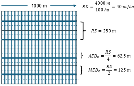
Fig. 1. Theoretical illustration of an ideal case of forest area of 100 ha, with 4 straight forest roads, mean road spacing (RS) of 250 m, road density (RD) of 40 m ha–1, calculative average extraction distance (AED0) of 62.5 m and calculative maximum extraction distance (MED0) of 125 m.
Backmund’s accessibility index E expresses how efficiently the existing road network expressed with calculative maximum extraction distance, MEDm is arranged compared to idealized layout. In mathematical form:

This type of comparison is easy to execute with modern GIS-based analytics. Fig. 2 demonstrates one example forest area from Central Finland, where existing forest road network in georeferenced vector format is derived from open-source databases maintained by the National Land Survey of Finland. In the given forest area of 2456 hectares, an existing road network of 62 406 m, resulting in a road density of 25.4 m ha–1. Road spacing is then approximately 400 m. With MED0 of 200 m wide buffer, a GIS software procedures output a polygon which cumulative net coverage is 1739 ha. The accessibility index E is then:

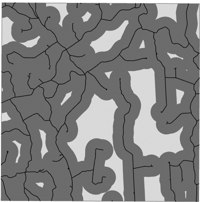
Fig. 2. A forest area of 2456 ha from Central Finland having forest roads of 62 406 m (25.4 m ha–1). With MED0 of 200 m (~RS/2), the accessibility index E = 0.708. The black vector line describes road network and dark grey the 200 m buffer around the road lines. Light grey describes the forest area that cannot be accessed with the MED0 of 200 m from the closest road.
Lünzmann (1968) continued the work of Backmund (1966) and demonstrated how the layout accessibility index can be used in highlighting areas where new roads should be placed. He stressed that one single metric can give a rather oversimplified picture about performance of the road network since it treats very different network flaws as equivalent. He emphasized that road orientation and geometry have a strong influence on the effective service corridor. He suggested that the forest area should be split into several subareas and the efficiency of the network should be examined in each subarea individually. He proposed that the efficiency of the layout should be assessed with an accessibility factor KE which is the inverse of E:

The given metrics describe the same phenomenon but from opposite perspectives. Factor KE has a penalty perspective (i.e. how much worse is my real network compared to the ideal one), whereas E describes a performance perspective (i.e., how close am I to the ideal?). Correction factor KE typically receives values 1.0–2.0 in subareas although Lünzmann (1968) showed that in some restricted areas 0.95 can be achieved with fork type road layout. Backmund (1966) outlined that the E of road layouts in Germany typically varies 0.65–0.80.
Both authors admitted that the calculative average and maximum values do not appear in real life since wood is not extracted along a straight line to the closest point of the road network. Instead, to get a realistic estimate for mean and maximum distances the calculative average and maximum values should be multiplied with a separate terrain factor Tcor. Based on the earlier inventories carried out in Sweden, Tcor can vary 1.0–2.0, mean value being roughly 1.35–1.40 (Segebaden 1964). The correction factor of 1.4 has later been applied also in Finnish road layout studies (Viitala and Uotila 1999; Uotila and Viitala 2000). Similarly, Backmund (1966) proposed a Tcor of  . He showed that the calculative average extraction distance multiplied with the Tcor is in line with the observations inventoried in real forest operations. Hence, the realistic average extraction distance AEDt can be calculated with Eq. 5:

In our example forest (Fig. 2), we got:

2.2 Quantitative metrics of the logging trail network
Metrics that analyse quantitative aspects of the logging trail network are derived from two spatial features: a polyline representing the centerline of the logging trail network and a polygon defining the boundaries of the logging site. Intersections or junctions where two trails cross or merge are referred to as nodes. The portion of a polyline between two nodes is defined as a segment. The polyline may also store attribute information, such as the number of times a given segment within the network has been traversed. From the given logging trail network polyline and stand polygon we can compute the following quantitative metrics:
TL: Logging trail network length (m), derived from the logging trail network polyline.
Atot: Area (m2) of the logging site polygon.
TD: Logging trail network density (m ha–1).
TSn: Nominal logging trail spacing (m) (similar to Eq. 1).

DIST: Distance travelled (m), calculated as the sum of segment lengths multiplied by the number of machine passes.
In addition, we can create buffer polygon regions around the logging trail polylines and evaluate pairwise buffer intersections in order to identify areas where two or more buffers overlap. Based on these operations, the following metrics are derived:
AT: Logging trail area (m2), calculated as TL multiplied by the nominal trail width (e.g., 4.5 m).
AT%: Proportion of trail area within the logging site (%), calculated as AT/Atot.
ANBRC: Net boom reach coverage (m2), defined as the total area reachable within the nominal crane length (~10 m). Areas extending beyond the logging site polygon are clipped.
ATSC: Net coverage (m2) reached with the nominal logging trail spacing (TSn).
2.3 Spatial configuration metrics of the logging trail network
Backmund (1966) based his accessibility index on calculative average and maximum distances. The calculated values are, however, only mean values. The metrics do not specifically penalize if any value exceeds a certain point. There is actually no constraint on how large the transportation distance can be. In efficiently managed forests, we aim at trail spacing of 20 m which means that all trees can be reached with a 10 m crane from the trail. In this type of context, we want to achieve minimum trail length distance (maximum trail length efficiency) while simultaneously controlling too small or too long distance between adjacent trails.
In forest conditions where trail spacing must be maintained within crane reach (circa 20 m), we propose a framework for assessing the spatial performance of the logging trail layouts using two coefficients: a Coverage Coefficient and a Structural Efficiency Coefficient.
The Coverage Coefficient, CA, measures the share of the forest area that is reachable by the modern harvester. In mathematical form:

It would be favourable to have a high Coverage Coefficient, but it can also be reached with a dense but wasteful trail network. Therefore, we need to also compare actual trail length to the ideal network. Similarly to Eq. 1 and illustrations given in Fig. 1, the density of the ideal logging trail network, TD0 (m ha–1) can be defined as:

where TS0 is the ideal logging trail spacing (m).
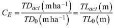
The Structural Efficiency Coefficient, CE, compares the actual trail length, TLact, to the ideal trail length, TL0, or actual trail length density, TDact, to the ideal trail length density, TD0. In mathematical form:

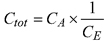
It is also possible to combine these two coefficients defined above. Since CA ≤ 1 and CE ≥ 1 (in most cases), a meaningful Structural-Coverage Efficiency index (Ctot) that combines these two coefficients for any logging trail network can be computed as:

In the forest with wider spacing (30–40 m) – where the trees beyond the nominal reach are intentionally left unharvested or treated by directional felling or winches – we propose that the quality of the layout is assessed with the metrics proposed by Backmund (1966) as follows:

An approximation of Eq. 12 can also more simply be attained with Eq. 9. Both indicates the share of forest reached with the nominal mean spacing compared to the ideal layout.
2.4 Geometrically corrected average logging trail spacing
In practical operations, machine operators strive for an ideal network layout by keeping the actual spacing between adjacent trails as close to optimal as possible, by avoiding building unnecessary junctions and by keeping the crossing angles as close to perpendicular as possible. With the logging trail polylines, we can also assess the spatial arrangement performance of the layout by calculating the average distance between adjacent, non-intersecting logging trails. The procedure for calculating geometry-corrected average trail distances is outlined as follows:
A. Grouping of trails (segments)
Trails are first divided into groups based on their orientations using the K-means algorithm. At this point small segment lines (less than 20 m) are removed (Fig. 3). Each group is processed independently to avoid mixing trails that are not spatially comparable. Only groups containing at least two trails are analysed.
B. Selection of a starting trail
Within each group, one trail is selected as the starting reference. The selection depends on the group and is based on spatial position (e.g., upper-left or lower-left corner of the group extent). This ensures a consistent traversal direction when iterating through adjacent trails.
C. Identification of the nearest non-intersecting trail
From the remaining trails in the group, the algorithm identifies the trail that:
• Does not intersect the current trail, and
• Has the smallest Euclidean distance to it.
This nearest non-intersecting trail is assumed to be the adjacent trail for spacing calculation.
D. Estimation of the local tangent on the adjacent trail
To account for trail curvature, spacing is not measured to the entire trail geometry but instead to a local tangent line:
• The point on the adjacent trail closest to the current trail is identified.
• The local direction of the trail near that point is approximated using neighbouring vertices.
• A straight line (tangent) is fitted through this local segment.
This tangent line represents the local orientation of the adjacent trail at the point of closest approach.
E. Sampling points on the current trail
To avoid bias from a single distance measurement:
• Several equally spaced points (typically three; they can be changed in the code) are sampled along the current trail.
• These points represent different positions along the trail length.
F. Perpendicular distance calculation
For each sampled point:
• The perpendicular distance to the tangent line of the adjacent trail is calculated.
• This yields multiple distance estimates for the same trail pair (see Fig. 4).
The perpendicular distance is used because it represents the true shortest spacing between approximately parallel trails.
G. Averaging distance for a trail pair
The mean of the perpendicular distances from all sampled points is computed.
This value represents the average spacing between the two adjacent trails. To exclude unrealistic or erroneous matches (e.g., distant or unrelated trails), distances larger than a predefined threshold (40 m) are discarded.
H. Iterative processing of all trails
The adjacent trail becomes the new reference trail, and the process repeats:
• Nearest non-intersecting trail is identified,
• Local tangent is fitted,
• Distances are sampled and averaged.
This continues until all trails in the group have been processed.
I. Calculation of group-level and total values for average distance
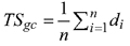
For each group independently and for all groups, the final average distance between the trails (TSgc = Geometry-corrected average trail spacing) is calculated as:

where di is the average spacing between two adjacent trails, and n is the number of valid adjacent trail pairs.
The logging trail network metrics presented in this chapter are summarized in Table 1.
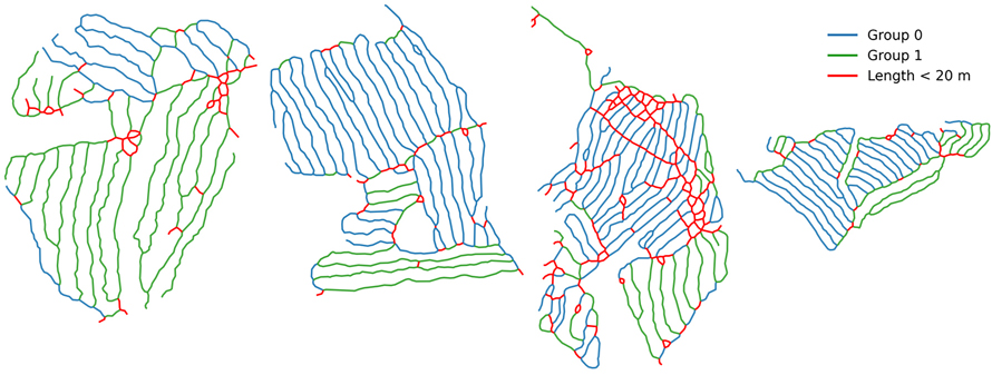
Fig. 3. Illustration of grouping of segments. Small line segments (<20 m) are removed (red-coloured segments). Remaining line segments are grouped based on their orientation using the K-means algorithm (blue and green coloured segments).
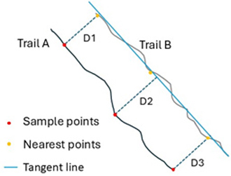
Fig. 4. Illustration of the distance calculation between adjacent trails.
| Table 1. Summary of the logging trail network metrics. | |||
| Definition | Equation | ||
| Metrics that analyse quantitative aspects of the logging trail network | TL | Logging trail network length (m), derived from the logging trail network polyline | |
| Atot | Area (m2) of the logging site polygon | ||
| TD | Logging trail network density (m ha–1) | ||
| TSn | Nominal logging trail spacing (m) | ||
| DIST | Distance travelled (m), calculated as the sum of segment lengths multiplied by the number of machine passes | ||
| Quantitative metrics considering buffer polygon regions | AT | Logging trail area (m2), calculated as TL multiplied by the nominal trail width (e.g., 4.5 m) | |
| AT% | Proportion of trail area within the logging site (%), calculated as AT/Atot | ||
| ANBRC | Net boom reach coverage (m2), defined as the total area reachable within the nominal crane length (~10 m). Areas extending beyond the logging site polygon are clipped | ||
| ATSC | Net coverage (m2) reached with the nominal logging trail spacing (TSn) | ||
| Spatial configuration metrics of the logging trail network | CA | Measures the share of the forest area that is reachable by the modern harvester | |
| TD0 | The density of the ideal logging trail network | ||
| CE | Compares the actual trail length, TLact, to the ideal trail length, TL0, or actual trail length density, TDact, to the ideal trail length density, TD0 | ||
| Ctot | Structural-Coverage Efficiency index. Combines coefficients CA and CE | ||
| TSgc | Average logging trail spacing | ||


3 Tests with real data
Harvesters and forwarders currently operating in Finnish forests are equipped with standard single-frequency GNSS receivers and antennas. We obtained a dataset of GNSS track vectors and forest stand polygons from Metsä Group covering ten forest sites located in Central Finland (the municipalities of Virrat and Ruovesi). These sites were harvested during thinning operations in the winter of 2024, following standard Finnish forest management recommendations. These recommendations specify both the recommended and minimum residual standing volumes after harvesting, as well as a target mean spacing of approximately 20 m between machine trails.
We did not receive any information regarding the type of GNSS receivers used or the manufacturers of the machines. Moreover, the process by which the original GNSS point observations were converted into vector tracks is unknown. Each machine route creates a separate GNSS track. Repetitive traffic along the same trail appears as a cluster of fuzzy lines, with no precise definition of the logging trail centerline.
Consolidated centerlines for the actual logging trail network were constructed with the procedures proposed by Cao et al. (2025). The procedures also create an estimate for the number of machine passes for each segment of the network. The system is based on the Kernel-density estimation method which goal is to create a smooth approximation of the underlying distribution. The bandwidth (search radius) plays a crucial role in this process. It determines the width of the area around each data point where the Kernel function is applied. In the next step, the Kernel-density raster is converted to a binary raster. At this stage, low density areas are cut off by adjusting the threshold value, typically being between 0.75–0.90.
The original datasets showed large deviations in the number of machine passes and horizontal discrepancies among tracks representing the same trail. Forest contractors are typically instructed to maintain a GNSS receiver and store GNSS track files in both harvesters and forwarders. We examined the GNSS tracks in the databases and found that, at many sites, forwarder GNSS tracks were partially or completely missing. Due to the deviations in the original datasets, we fine-tuned, for each site separately, the values of the most important parameters controlling the conversion process, namely the kernel density smoothing radius and the trail area thresholding value (Table 2). For other parameters, we employed the values proposed by Cao et al. (2025) (Table 1). Based on these estimations of the logging trail network polyline, we computed the quantitative and qualitative logging trail network metrics presented in Section 2 using Python libraries.
| Table 2. Estimation of GNSS tracks per logging trail segment and the parameter values employed to consolidate the centerline (based on the algorithms by Cao et al. 2025). | ||||||
| Stand | No. of tracks per logging trail segment | Origin of GNSS Tracks H = harvester H+F = harvester and forwarder | Kernel density search radius | Threshold value | ||
| No. | Min | Max | Most frequent | |||
| 1 | 1 | 5 | 2 | H | 1.5 | 0.70 |
| 2 | 1 | 14 | 4 | H+F | 1.5 | 0.70 |
| 3 | 1 | 14 | 14 | H+F | 0.65 | 0.85 |
| 4 | 1 | 14 | 2 | H+F | 1.5 | 0.70 |
| 5 | 1 | 5 | 2 | H | 2.5 | 0.80 |
| 6 | 1 | 5 | 2 | H | 1.5 | 0.70 |
| 7 | 1 | 14 | 6–7 | H+F | 2 | 0.80 |
| 8 | 1 | 8–9 | 2 | H+F | 2.5 | 0.80 |
| 9 | 1 | 14 | 6–7 | H+F | 1.5 | 0.70 |
| 10 | 1 | 14 | 4 | H+F | 1.5 | 0.70 |
The compatibility of the logging trail networks and site polygons was verified by examining the logical consistency of these layers using GIS. At this stage, a corner of one original polygon was removed, as no evidence of machine traffic or harvesting operations was observed in that area.
A custom software script was developed to read the processed centerline polylines and the corresponding forest site boundary polygon for each stand individually, and to compute the metrics presented in Chapter 2. An illustration of part of logging site 1 is shown in Fig. 5, depicting the logging trail centerline, net and gross boom reach coverage buffers (with a boom reach of 10 m), and the logging trail area, represented by a 2.25 m centerline buffer corresponding to a nominal trail width of 4.5 m.
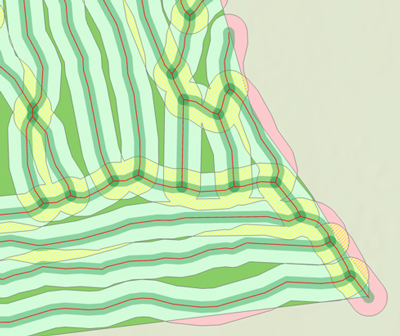
Fig. 5. Part of logging site 1. The site polygon is shown in dark green, the 10 m buffer around the logging trails in light green, and the logging trail area in medium green. Yellow areas indicate overlaps of the boom reach, while red areas represent boom reach extending outside the stand polygon.
4 Results
In most stands, operators have managed to create a network layout that can be regarded as moderate (stands 5, 6, 7 and 9) or very good (stands 1, 2 and 10) (Table 3). At the best sites (see Fig. 6a, stand 10), trail density is close to 500 m ha–1, the Structural Efficiency Coefficient (CE) is close to 1 and the Coverage Coefficient (CA) is at a moderate level.
Metrics from stands 3, 4 and 9 indicate that the network layout deviates from the ideal. In these stands, trail density is approximately 600 m ha–1 or higher, and the Structural Efficiency Coefficient (CE) ranges from 1.2 to 1.3 (see Fig. 6b, stand 4). However, it should be noted that no factors potentially affecting these results were investigated. The sites may include obstacles or constraints (e.g. steep slopes, stoniness, wetness, ditches, or old trails) that could have influenced the layout. A correlation analysis was conducted using the values in Table 3. Only one notable relationship was identified: the geometrically corrected average trail spacing (TSgc) shows a moderate correlation with the structural efficiency coefficient (CE) and the combined index (Structural-Coverage Efficiency index) (Fig. 7). This indicates that TSgc may also serve as an indicator of layout efficiency.
| Table 3. Summary of logging trail network metric values by sample stand. | |||||||||
| Stand No. | Stand area Atot ha | Trail length TL m | Trail density TD m ha–1 | Trail spacing TSgc m | Share of trail area AT% | Net boom reach coverage ANBRC m2 | Coverage Coefficient CA | Structural Efficiency CE | Structural – Coverage Efficiency index Ctot = CA × CE–1 |
| 1 | 13.4 | 6558 | 487 | 20.0 | 21.4 | 10.9 | 0.81 | 0.98 | 0.83 |
| 2 | 19.8 | 9561 | 482 | 20.8 | 21.4 | 16.6 | 0.84 | 0.97 | 0.87 |
| 3 | 10.5 | 6244 | 594 | 20.3 | 25.7 | 19.0 | 0.87 | 1.19 | 0.73 |
| 4 | 13.9 | 9077 | 652 | 16.9 | 27.8 | 11.8 | 0.85 | 1.30 | 0.65 |
| 5 | 26.6 | 14292 | 537 | 21.4 | 23.7 | 23.2 | 0.87 | 1.07 | 0.81 |
| 6 | 7.83 | 4220 | 538 | 23.0 | 23.9 | 6.89 | 0.88 | 1.08 | 0.81 |
| 7 | 1.68 | 950 | 566 | 20.0 | 24.9 | 1.54 | 0.92 | 1.13 | 0.81 |
| 8 | 4.62 | 2526 | 546 | 20.0 | 23.9 | 3.92 | 0.85 | 1.09 | 0.78 |
| 9 | 6.29 | 3801 | 604 | 19.4 | 26.6 | 5.74 | 0.91 | 1.21 | 0.75 |
| 10 | 13.1 | 6590 | 502 | 23.4 | 22.2 | 11.3 | 0.86 | 1.0 | 0.86 |
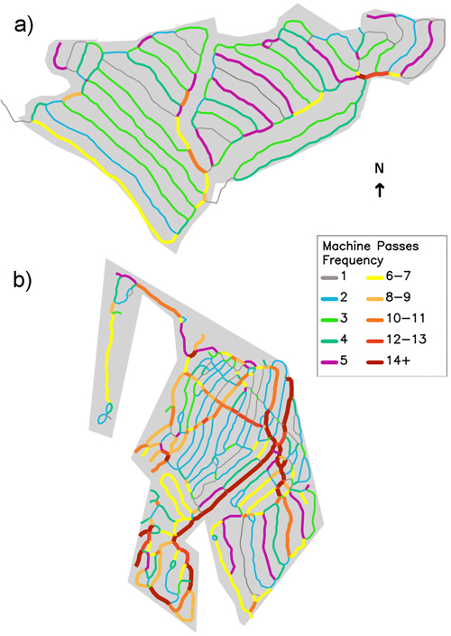
Fig. 6. Logging trail network of stand 10 (a), demonstrating a well-designed layout, and of stand 4 (b), demonstrating a poorly executed layout. Color-coding represents the number of machine passes.
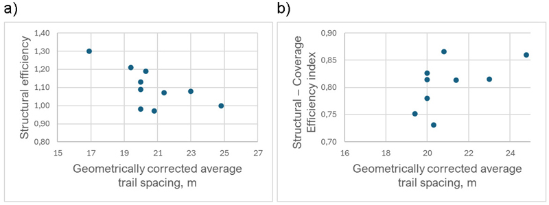
Fig. 7. In our small sample of ten sites, the geometrically corrected trail spacing (TSgc) was moderately correlated with the Structural Efficiency (r = –0.664, p = 0.036) (a) and with the Structural-Coverage Efficiency index (r = 0.753, p = 0.012) (b).
5 Discussion
In this work, we introduce a concept for assessing the spatial arrangement performance of the logging trail network. In efficiently managed forests, the target trail spacing is 20 m, which ensures that all trees can be reached with a 10 m crane from the trail. In this context, the objective is to minimize total trail length (i.e., maximize trail length efficiency) while simultaneously avoiding both excessively small and excessively large distances between adjacent trails.
We propose assessing the spatial arrangement performance of the logging trail network using two spatial configuration metrics: (1) a Coverage Coefficient, which defines the proportion of forest area reachable by a modern harvester, and (2) a Structural Efficiency Coefficient, which compares the actual trail length to the ideal trail length. The Coverage Coefficient ranges from 0to 1.0, whereas the Structural Efficiency Coefficient typically ranges from 1.0 to 2.0. The closer these values are to 1.0, the closer the network is to the ideal configuration.
In principle, these two metrics can be combined into a single indicator – the Structural–Coverage Efficiency Index – by multiplying the coverage coefficient by the inverse of the Structural Efficiency Coefficient. However, this approach may result in a loss of information regarding specific aspects of network spatial arrangement.
The methodology presented here is consistent with established targets for logging trail network design, namely maintaining inter-trail distances as close as possible to 20 m in all directions. This design objective inherently leads to high boom-reach coverage and minimal logging trail density.
Conceptually, in addition to the forest road design principles (Backmund 1966; Lünzmann 1968), the proposed Coverage Coefficient and Structural Efficiency Coefficient are analogous to normalized network efficiency measures used in urban street systems (Crucitti et al. 2006; Barthélemy 2011) and to area coverage metrics applied in wireless sensor networks (Huang and Tseng 2005). They also share similarities with studies on agricultural machinery that aim to optimize path spacing (Bochtis and Vougioukas 2008; Hameed et al. 2013).
We also introduce a method for calculating a geometrically meaningful mean spacing between adjacent trails. Using classical mathematical approaches, average trail spacing is typically derived from overall trail density. While this can yield numerically sound mean spacing values, the resulting trail distribution may be geometrically uneven and therefore practically unacceptable.
The geometrically corrected mean spacing provides a meaningful way to assess the spatial arrangement performance of the logging trail network and is strongly aligned with the practical instructions given to machine operators. Moreover, controlling the mean distances of the logging trail network using a single, simple metric has clear advantages, as it is easier to comprehend than approaches based on multiple metrics.
However, the proposed method also has limitations. If the network comprises a large number of short trail segments – particularly segments shorter than 20 m – the metric may yield results that do not fully describe the overall performance of the design. It should also be noted that the procedures used to create trail centerlines (Cao et al. 2025) do not always produce a perfect representation of the actual trail network.
The metrics developed and described here were tested using datasets derived from ten forest sites located in Central Finland. The number of sites is small, and therefore we cannot guarantee that the selected sites fully represent the variation of the broader population of thinning operations in Finland. Moreover, no data were collected on factors that may have influenced trail network design, such as steep slopes, stoniness, soil wetness, ditches, protected areas, or pre-existing trails.
For these reasons, no definitive conclusions can be drawn regarding the overall success of logging trail design in this region. The data do indicate, however, that differences exist in layout performance among sites, and the metrics presented here provide a useful starting point for assessing the differences in spatial arrangement.
Having a robust spatial configuration metric for logging trail networks is important for several reasons. First, a well-defined metric provides feedback to machine operators and helps them improve their decision-making and work processes when operating in new sites. Moreover, the same information can be communicated to forest owners and authorities who may be interested in the qualitative aspects of harvesting operations.
Second, a reliable metric plays an important role in reducing CO₂ emissions. A non-optimal logging trail network length affects work efficiency, wood production, and the forest carbon balance. According to our findings, logging trail network density in Finnish forests after first thinning ranges from 480 to 700 m ha⁻1, with an average of approximately 580 m ha⁻1. Reducing network density by 10% could decrease energy consumption per harvested volume by about 5%, achieved through shorter forwarding distances and improved harvesting efficiency. Increased logging trail network density also influences harvesting intensity and future wood production. It is well established that thinning strongly affects post-harvest volume increment of retained trees; however, if thinning is too intensive, increased growth cannot compensate for the loss in carbon sequestration relative to an optimally thinned forest. Heavy thinning therefore results in lower total carbon accumulation over the rotation period.
Third, recent scientific efforts to develop automated trail network design and planning (TNDP) procedures require metrics that can guide optimization. Although TNDP solutions may include multiple objectives (Holmström et al. 2023), optimizing trail network length and overall network quality remains one of the most important goals of any such optimization procedure.
A prerequisite for applying the metrics presented in this study is the availability of reliable data on the positions of logging trails. This condition is often not met; however, the situation is gradually improving. Recently, several methods have been proposed for deriving logging trail centerlines from GNSS data (Ovaskainen and Riekki 2022; Contreras et al. 2024; Cao et al. 2025). Based on these approaches, both quantitative and qualitative metrics can be calculated immediately after harvesting operations or even in near real time during operations. In addition, existing logging trail networks can be assessed prior to operations using remote sensing data (Abdi et al. 2022; Abdi and Uusitalo 2026). This enables operators to be better supported in planning how to complement and extend existing trail networks. We believe that the proposed spatial configuration metrics can support both pre-harvest planning of logging trail networks and post-harvest evaluation by providing feedback to machine operators and forest owners.
Spatial configuration metrics evaluate logging trail network design solely from the perspective of spatial arrangement. As such, they provide only a simplified indicator and do not account for several important factors. First, terrain topography can hinder or even completely prevent machine traffic. Wherever possible, logging trails should be located on stable ground with gentle slopes to ensure safe and efficient operations. Side slopes should be avoided because they increase the risk of machine rollover, while rocky terrain is often unsuitable due to the limited ground clearance of forest machines (approximately 50 cm). Second, forest machines are extremely heavy and may cause substantial soil disturbance if machine traffic is not restricted to less sensitive soil types (Sirén et al. 2019; Uusitalo et al. 2020). Third, environmental considerations related to biodiversity conservation and hydrology should guide both the placement of retention tree groups and the layout of logging trails. In boreal forests, large aspens, deadwood, and structural heterogeneity are particularly important indicators of biodiversity (Kivinen et al. 2020; Hämäläinen et al. 2024). Fourth, operational constraints on machine movement must be considered. Trail junctions should be gently curved, and the network should contain natural loops that allow machines to move through the stand without unnecessary turning or reversing maneuvers. Fifth, existing forest infrastructure may also influence trail network design. In previously managed forests, existing logging trails should be taken into account during planning, as disregarding them may result in unnecessary harvesting of residual trees and an excessive density of new trails (Abdi et al. 2022; Abdi and Uusitalo 2026).
Data statement
The GNSS tracks were collected by a number of individual contractors working in private forests. These data cannot be shared with third parties.
Software
The code and anonymized example datasets are available in the GitHub repository: https://github.com/forest-technology-helsinki/logging-trail-analyzer.
Authors’ contributions
JU, ZM, SC, OA: Conceptualization, methodology, interpretation of data, software development, visualization; JU: funding acquisition, project administration, acquisition of data, compiling complete draft; JU, ZM, SC, OA: Revising the final manuscript.
Acknowledgements
We would like to thank Metsä Group for providing us with the GNSS data tracks from their archives.
Funding
This work was funded by the Next Generation EU/RRF programme through a grant from the Ministry of Agriculture and Forestry of Finland (decision number VN/32537/2021) and was also supported by the OptiForValue project (No. 101157658), funded by the CBE JU under powers delegated by the European Commission.
Declaration of generative AI and AI-assisted technologies in the manuscript preparation process
During the preparation of this work the author(s) used ChatGPT 4.0 in order to polish some part of the text. After using this tool/service, the authors reviewed and edited the content as needed and take full responsibility for the content of the publication.
References
Abdi O, Uusitalo J (2026) High-Resolution GeoAI framework for automated rutting depth prediction on logging trails using TransRAUnet and LiDAR. Comput Electron Agric 245, article id 111547. https://doi.org/10.1016/j.compag.2026.111547.
Abdi O, Uusitalo J, Kivinen V-P (2022) Logging trail segmentation via a novel U-Net convolutional neural network and high-density laser scanning data. Remote Sens 14, article id 349. https://doi.org/10.3390/rs14020349.
Backmund F (1966) Kennzahlen für den Grad der Erschliegung yon Forstbetrieben durch autofahrbare Wege. Forstw Cbl 85: 342–354. https://doi.org/10.1007/BF02202207.
Barthélemy M (2011) Spatial networks. Phys Rep 499: 1–101. https://doi.org/10.1016/j.physrep.2010.11.002.
Bochtis DD, Vougioukas SG (2008) Minimising the non-working distance travelled by machines operating in a headland field pattern. Biosyst Eng 101: 1–12. https://doi.org/10.1016/j.biosystemseng.2008.06.008.
Cao S, Abdi O, Koivukoski K, Mao Z, Uusitalo J (2025) Automating the consolidation of GNSS logging tracks and machine pass counting in boreal forests. Smart Agric Technol 11, article id 101038. https://doi.org/10.1016/j.atech.2025.101038.
Contreras M, Parra C, Cárdenas C, Hermosilla C, Pastén R, Aedo D (2024) Skid trail network visualizer: a computational tool to generate skid trails created by ground-based timber harvesting machines and facilitate soil disturbance monitoring. Comput Electron Agric 225, article id 109282. https://doi.org/10.1016/j.compag.2024.109282.
Contreras MA, Parrott DL, Chung W (2016) Designing skid-trail networks to reduce skidding cost and soil disturbance for ground-based timber harvesting operations. For Sci 62: 48–58. https://doi.org/10.5849/forsci.14-146.
Contreras MA, Parrott DL, Stringer JW (2020) Retroactive comparison of operator-designed and computer-generated skid-trail networks on steep terrain. For Syst 29, article id eSC01. https://doi.org/10.5424/fs/2020291-15558.
Crucitti P, Latora V, Porta S (2006) Centrality measures in spatial networks of urban streets. Phys Rev E 73, article id 36125. https://doi.org/10.1103/PhysRevE.73.036125.
Flisberg P, Rönnqvist M, Willén E, Frisk M, Friberg G (2021) Spatial optimization of ground-based primary extraction routes using the BestWay decision support system. Can J For Res 51: 675–691. https://doi.org/10.1139/cjfr-2020-0238.
Froehlich HA, Aulerich DE, Curtis R (1981) Designing skid trail systems to reduce soil impacts from tractive logging machines. Research Paper 44. Forest Research Laboratory, School of Forestry, Oregon State University, Corvallis, OR, USA.
Garland JJ (1983) Designated skid trails minimize soil compaction. Forest Research Laboratory, School of Forestry, Oregon State University, Extension Service, Corvallis, OR, USA.
Gumus S, Turk Y (2016) A new skid trail pattern design for farm tractors using linear programing and geographical information systems. Forests 7, article id 306. https://doi.org/10.3390/f7120306.
Hämäläinen A, Runnel K, Ranius T, Strengbom J (2024) Diversity of forest structures important for biodiversity is determined by the combined effects of productivity, stand age, and management. Ambio 53: 718–729. https://doi.org/10.1007/s13280-023-01971-9.
Hameed IA, Bochtis DD, Sørensen CG, Jensen AL, Larsen R (2013) Optimized driving direction based on a three-dimensional field representation. Comput Electron Agric 91: 145–153. https://doi.org/10.1016/j.compag.2012.12.009.
Holmström E, Nikander J, Backman J, Väätäinen K, Uusitalo J, Jylhä P (2023) A multi-objective optimization strategy for timber forwarding in cut-to-length harvesting operations. Int J Forest Eng 34: 267–283. https://doi.org/10.1080/14942119.2022.2149003.
Hosseini A, Lindroos O, Wadbro E (2019) A holistic optimization framework for forest machine trail network design accounting for multiple objectives and machines. Can. J. For. Res. 49:111–120. https://doi.org/10.1139/cjfr-2018-0258.
Hosseini A, Wadbro E, Ngoc Do D, Lindroos O (2023) A scenario-based metaheuristic and optimization framework for cost-effective machine-trail network design in forestry. Comput Electron Agric 212, article id 108059. https://doi.org/10.1016/j.compag.2023.108059.
Huang C-F, Tseng Y-C (2005) The Coverage Problem in a Wireless Sensor Network. Mobile Netw Appl 10: 519–528. https://doi.org/10.1007/s11036-005-1564-y.
Jacob M, Cremer T, Mederski PS, Ferréol B (2026) Productivity, costs and residual stand damage of timber harvesting methods in Scots pine stands with extended distance between skid trails. Croat J For Eng 47: 69–87. https://doi.org/10.5552/crojfe.2026.4081.
Kivinen S, Koivisto E, Keski-Saari S, Poikolainen L, Tanhuanpää T, Kuzmin A, Viinikka A, Heikkinen RK, Pykälä J, Virkkala R, Vihervaara P, Kumpula T (2020) A keystone species, European aspen (Populus tremula L.), in boreal forests: ecological role, knowledge needs and mapping using remote sensing. For Ecol Manag 462, article id 118008. https://doi.org/10.1016/j.foreco.2020.118008.
Lotfalian M, Khosrozadeh S, Hosseini SA, Kazemi M, Zare N (2016) Determination of forest skid trail density in Caspian forests, Iran. J For Sci 62: 80–87. https://doi.org/10.17221/84/2015-JFS.
Lünzmann K (1968) Der Erschliessungskoeffizient, eine Kennzahl zur Beurteilung von Waldwegenetzen und seine Anwendung bei Neuplanungen. Forstw Cbl 87: 237–248. https://doi.org/10.1007/BF02735865.
Mederski PS (2006) A comparison of harvesting productivity and costs in thinning operations with and without midfield. For Ecol Manag 224: 286–296. https://doi.org/10.1016/j.foreco.2005.12.042.
Ovaskainen H, Riekki K (2022) Computation of strip road networks based on harvester location data. Forests 13, article id 782. https://doi.org/10.3390/f13050782.
Segebaden G von (1964) Studies of cross-country transport distances and road net extension. Stud For Suec 18: 8–69. https://pub.epsilon.slu.se/12770/1/SFS018.pdf.
Sirén M, Salmivaara A, Ala-Ilomäki J, Launiainen S, Lindeman H, Uusitalo J, Sutinen R, Hänninen P (2019) Predicting forwarder rut formation on fine-grained mineral soils. Scand J For Res 34: 145–154. https://doi.org/10.1080/02827581.2018.1562567.
Søvde NE, Løkketangen A, Talbot B (2013) Applicability of the GRASP metaheuristic method in designing machine trail layout. For Sci Technol 9: 187–194. https://doi.org/10.1080/21580103.2013.839279.
Uotila E, Viitala E-J (2000) Tietiheys metsätalouden maalla. [Forest road density in forestry land]. Metsätieteen aikakauskirja 1/2000: 19–33. https://doi.org/10.14214/ma.6910.
Uusitalo J (2010) Introduction to forest operations and technology. JVP Forest Systems Oy. ISBN 978-952-92-5269-5.
Uusitalo J, Ala-Ilomäki J, Lindeman H, Toivio J, Sirén M (2020) Predicting rut depth induced by an 8-wheeled forwarder in fine-grained boreal forest soils. Ann For Sci 77, article id 42. https://doi.org/10.1007/s13595-020-00948-y.
Viitala E-J, Uotila E (1999) Optimaalinen tietiheys yksityismetsätalouden kannalta. [Optimal road density in Finnish private forestry]. Metsätieteen aikakauskirja 2/1999: 167–179. https://doi.org/10.14214/ma.6117.
Werder M, Bont LG, Schweier J, Thees O (2025) A comprehensive analysis of time investment in skid trail planning for forest access. PLoS One 20, article id e0317963. https://doi.org/10.1371/journal.pone.0317963.
Total of 34 references.

