Lauri Korhonen  ,
Inka Pippuri,
Petteri Packalén,
Ville Heikkinen,
Matti Maltamo,
Juho Heikkilä
,
Inka Pippuri,
Petteri Packalén,
Ville Heikkinen,
Matti Maltamo,
Juho Heikkilä
Detection of the need for seedling stand tending using high-resolution remote sensing data
Korhonen L., Pippuri I., Packalén P., Heikkinen V., Maltamo M., Heikkilä J. (2013). Detection of the need for seedling stand tending using high-resolution remote sensing data. Silva Fennica vol. 47 no. 2 article id 952. https://doi.org/10.14214/sf.952
Abstract
Seedling stands are problematic in airborne laser scanning (ALS) based stand level forest management inventories, as the stem density and species proportions are difficult to estimate accurately using only remotely sensed data. Thus the seedling stands must still be checked in the field, which results in an increase in costs. In this study we tested an approach where ALS data and aerial images are used to directly classify the seedling stands into two categories: those that involve tending within the next five years and those which involve no tending. Standard ALS-based height and density features, together with texture and spectral features calculated from aerial images, were used as inputs to two classifiers: logistic regression and the support vector machine (SVM). The classifiers were trained using 208 seedling plots whose tending need was estimated by a local forestry expert. The classification was validated on 68 separate seedling stands. In the training data, the logistic model’s kappa coefficient was 0.55 and overall accuracy (OA) 77%. The SVM did slightly better with a kappa = 0.71 and an OA = 86%. In the stand level validation data, the performance decreased for both the logistic model (kappa = 0.38, OA = 71%) and the SVM (kappa = 0.37, OA = 72%). Thus our approach cannot totally replace the field checks. However, in considering the stands where the logistic model predictions had high reliability, the number of misclassifications reduced drastically. The SVM however, was not as good at recognizing reliable cases.
Keywords
forest management;
airborne laser scanning;
logistic regression;
seedling stand;
tending;
support vector machine
-
Korhonen,
School of Forest Sciences, University of Eastern Finland, P.O. Box 111, FI-80101 Joensuu, Finland
E-mail
lauri.korhonen@uef.fi
- Pippuri, School of Forest Sciences, University of Eastern Finland, P.O. Box 111, FI-80101 Joensuu, Finland E-mail inka.pippuri@uef.fi
- Packalén, School of Forest Sciences, University of Eastern Finland, P.O. Box 111, FI-80101 Joensuu, Finland E-mail petteri.packalen@uef.fi
- Heikkinen, School of Computing, University of Eastern Finland, P.O. Box 111, FI-80101 Joensuu, Finland E-mail ville.heikkinen@uef.fi
- Maltamo, School of Forest Sciences, University of Eastern Finland, P.O. Box 111, FI-80101 Joensuu, Finland E-mail matti.maltamo@uef.fi
- Heikkilä, Finnish Forest Centre, Public Services, Maistraatinportti 4 A, FI-00240 Helsinki, Finland E-mail juho.heikkila@metsakeskus.fi
Received 20 December 2012 Accepted 14 March 2013 Published 25 June 2013
Views 144221
Available at https://doi.org/10.14214/sf.952 | Download PDF

Abbreviations
| AGL | Above ground level |
| ALS | Airborne laser scanning |
| CV | Cross validation |
| GFFS | Greedy forward feature selection |
| NIR | Near-infrared band in an aerial image |
| NDVI | Normalized difference vegetation index |
| OA | Overall accuracy (percent of correctly classified instances) |
| RED | Red band in an aerial image |
| RS | Remote sensing |
| SR | Simple ratio |
| SVM | Support vector machine (classifier) |
1 Introduction
In Finland, forests cover 70% of the land area and thus the forestry sector is economically important. Efficient forest management is encouraged in order to maintain the timber supply for the forest industries. Forest regeneration is one the most important parts of even-aged forest management, because the success of regeneration largely defines the development of forest stands during forest rotation. The aim of the process is to create a vital seedling stand that has an appropriate density of high-quality seedlings with suitable species composition and a regular spatial pattern. The Finnish Forest Act (1996/1039) requires that an economically developable seedling stand must be established in a reasonable time and must not be immediately disturbed by other vegetation. The development of a productive tree stand is ensured by the cleaning of disruptive vegetation and by pre-commercial thinning to a suitable growth density (Tapio 2006). Determining the need and proper timing for the tending of seedling stands has a large impact on the growth and dynamics of the tree stand, as well as for the profitability of the first commercial thinning (e.g. Huuskonen and Hynynen 2006; Uotila et al. 2011). Nevertheless, seedling stand tending is often neglected by private forest owners.
Seedling stands are defined as having mean height < 7 m (conifer) or 9 m (deciduous), and are often further divided into young (< 1.3 m) and advanced (1.3–7 or 9 m) seedling stands (Tapio 2006). The assessment of regeneration is based on field measurements of stem density, tree height, and a visual field assessment of seedling condition, species proportions and the spatial pattern of trees. This information is used for determining the need for active treatments in the near future. The official guidelines (Tapio 2006) recommend early tending at the height of 1–2 meters, which has to be performed if the competing species or weeds start to hinder the main species’ growth. In early tending, only the competing vegetation is removed. The proper tending takes place at a height of 5–7 meters, when the remaining tree population is thinned to a density of approximately 1500–2500 trees per hectare.
Concerns over the success of forest regeneration and demands to decrease the costs of stand level forest management inventories have created a need for developing more efficient methods for assessing forest regeneration. Remote sensing (RS) based forest inventory methods have been studied intensively and adopted into practical use in many countries. However, the seedling stands are difficult targets for remote sensing because of the small size of the crowns and their clustered spatial arrangement (Hall and Aldred 1992). The first experiments in RS-based seedling stand inventory were made using optical remote sensing techniques. For example, Pesonen et al. (2007) assessed the need for the tending of seedling stands based on the proportion of deciduous trees using a combined map of Landsat TM -satellite images and field data from the Finnish National Forest Inventory. The overall accuracy (OA) in mineral soils was 62%. Hyvönen (2002) studied the suitability of Landsat TM images to estimate silvicultural operations with a data including both seedling stands and young forests (OA = 76%). High-resolution aerial images have also been tested. Pouliot et al. (2002) obtained good results in the assessment of seedling stand tending needs using leaf-off aerial photographs with a 2-cm resolution. Such data is however too expensive for practical use. Tuomola et al. (2006) used textural features calculated from aerial images (scale 1:14 000) and forest stand information to estimate the seedling stand tending need. In their study, although aerial images did not adequately illustrate the need, the simultaneous use of image features and existing stand information improved the results.
Airborne laser scanning (ALS) is an RS technique that provides direct 3D-measurements of the earth surface and vegetation height. ALS echo heights are used to calculate features describing vegetation height and density for a set of satellite positioned field plots. Then it is possible to create models where the ALS features are used to predict different forest attributes such as growing stock volume, and use the models to create wall-to-wall maps of the inventory area (Næsset 2002). Spectral and textural features derived from aerial images are often used as additional predictors in the models, especially if species-wise predictions are needed (Packalén and Maltamo 2007). This approach is known as the area-based method, and it has been shown to enable determination of stand characteristics more accurately and with smaller costs than in traditional Finnish field inventory by compartments (Maltamo et al. 2011).
The potential of ALS in seedling stand inventories has been assessed in the Norway and Finland. Næsset and Bjerknes (2001) predicted tree height and the number of stems for seedling stands (height < 6 m) using low density ALS data and the area based method. The estimation of tree height was successful (R2 = 0.83), but the estimation of tree density was less accurate (R2 = 0.42). Närhi et al. (2008) obtained similar results for advanced spruce seedling stands with dominant heights of 2–8 meters using regression models based on sparse ALS data (stand density RMSE = 45%). They also assessed the need for tending (immediate, 1–5 years, no need) based on the field-measured stem density and height. Need for tending was predicted using two different techniques: 1) based on ALS features and forestry plan information using linear discriminant analysis 2) based on regression predictions of stand density and dominant height. The first approach yielded slightly better accuracies (OA = 72%, kappa = 0.54) than the second approach (OA = 69%, kappa = 0.34). Korpela et al. (2008) studied the combined use of ALS and airborne digital imagery in the classification of common seedling stand vegetation. The classification accuracy varied from 61.1% to 78.9% and they concluded that ALS is not applicable in classifying young seedling stands because of random errors in terrain and vegetation heights.
Tahvanainen (2011) used ALS features to determine the need for tending for the young seedling stands. For the advanced seedling stands, stand attributes such as stem density were predicted instead. The need for tending (0–5 years, no need) was evaluated in the field based on the official guidelines. The classification based on nearest neighbour models succeeded better for early tending of the young seedling stands (kappa = 0.68) than for proper tending of the advanced seedling stands (kappa = 0.58). Nivala (2012) used linear discriminant analysis to predict management need for seedling stands and young forests based on ALS features. Classification considered three classes: tending of seedling stands, fuel wood harvest at young forests, or no operations. Management need was assessed based on measured stand density, dominant height and thinning drain. The stands with management need were predicted more accurately (79% correct for seedling stands, 100% correct for young stands) than the stands with no need for operations (44% correct). The kappa-value of classification was 0.65.
In current operational ALS-based stand level forest management inventories, the seedling stand attributes (e.g. tree height, number of stems, species composition) are imputed by using the RS data in a similar manner as for mature stands. The tending need is then derived from the predicted attributes using general management guidelines (Tapio 2006). However, this approach has not produced adequate results. The main reason is that stand density and species composition are very difficult to assess with acceptable precision using RS data only. The estimated characteristics are averages and do not always describe the real need for operations, which would in practice be the most important information required to ensure the best possible stand development. In this case, it would be reasonable to determine the tending need, directly based upon ALS metrics. This approach has yielded some promising results for thinning (Vastaranta et al. 2011; Pippuri et al. 2012), but seedling stand tending has been more difficult to assess accurately (Närhi et al. 2008; Tahvanainen 2011; Nivala 2012).
The evaluation of tending needs of seedling stands is considered to be very important in maintaining future timber supply, and must be evaluated for all seedling stands in the new RS-based stand level forest management inventory system. As RS estimates have not been good enough, thus far, most seedling stands (typically 20–25% of the forestry land area) have still been evaluated in the field, although the interpretation of mature forests is based almost solely on the RS method. The total area of ALS-based forest inventory in private forests in Finland is 15 000–20 000 km2 annually. If the tending need could be predicted reliably for even some of the seedling stands without a field visit, then the total costs of the new inventory system would be considerably reduced. Some classifiers allow assessing the reliability of the predictions, and this information can be used to decide which stands do not need a field visit.
This research evaluates the use of high resolution remote sensing data in seedling stand inventory. We present our results concerning the estimation of stem density, as few international research papers have considered it this far. However, our main aim is to test direct classification of the seedling stands based on the RS data without predicting the other stand attributes. For this purpose, a total of 208 seedling plots were measured and a local expert defined the tending need for each plot. Features derived from digital aerial images and ALS data were used to classify the plots. We compared the performance of two commonly used classification methods, parametric logistic regression and non-parametric support vector machine. The predictions were evaluated in an independent validation of data consisting of 68 stands in the same area. We also analyzed the factors contributing to observed misclassifications, and studied how accurate the seemingly most reliable predictions actually were.
2 Materials and methods
2.1 Field data sets
The study area is located in Joutsa, central Finland (61°48ʹN, 26°5ʹE). The area has privately owned “semi-natural” boreal forests that are managed with varying intensity, dependent on the forest owner. The soils in the region are mostly very fertile, and the seedling stands must usually be tended several times in order to prevent the fast-growing deciduous species from shadowing the commercially important conifers. The most common tree species in the area are Scots pine (Pinus sylvesteris L.), Norway spruce (Picea abies L. Karst.), and birches (Betula spp. L.).
A total of 208 seedling plots were measured from 118 different stands in summer 2010. The seedling stands were selected based on aerial images from 2006 and existing stand information. Neither stands with mean height of less than 1.3 meters, nor stands taller than 9 meters were considered. One to three plots were located manually within each selected stand using GIS software. The plot positions were sought with a satellite positioning device. Sometimes the plot had to be moved from its intended position, for example if there were retention trees within the plot radius (9 m). The final position was recorded with Trimble GeoXH GPS, which has an accuracy better than one meter after a differential correction. The aim was to obtain a representative data set with different height, density and tending need classes for each of the main tree species in the area. Thus up to three plots were measured from stands that were not well represented in the data; in total, there were 53 stands with one plot, 40 stands with two plots, and 25 stands with three plots.
Common stand attributes such as stem density and the median tree characteristics of tree species were measured from each sample plot. The selection of trees that should be included into stem density measurements required some consideration, because understory trees are usually insignificant when the tending need is assessed. We decided to make a visual height assessment before any measurements were undertaken and only include trees that were taller than half of the estimated mean height. In the case of multi-stemmed species such as rowan (Sorbus aucuparia L.), all stems branching below 1.3 m were considered to be individual trees, which is the also the practice undertaken in the Finnish National Forest Inventory.
A key problem in direct tending need classification is how reliably it can be determined in the field. Unfortunately this is not a trivial issue. As mentioned above, early tending is recommended at the height of 1–2 meters, and proper tending at a height of 5–7 meters. However, the tending may need to be repeated several times if the competition of other species is intense. If early tending is neglected, the deciduous species will quickly suppress the conifers, which can lead to need for tending at any height. The evaluation of when the tending should be done is however very subjective and depends on the local conditions.
An experienced local forester estimated the tending need individually for each plot during the autumn of 2010 and before the growth season in spring 2011. The stands were initially classified into three classes: those needing immediate tending, those where tending was needed during the next 1–5 years, and those with no need for tending within the next ten years (Table 1).
| Table 1. The number of plots by tree species and tending need class in the training data. | ||||
| Main species | Need for tending | Total | ||
| Immediately | 1–5 years | No need | ||
| Scots pine | 12 | 37 | 55 | 104 |
| Norway spruce | 19 | 21 | 37 | 77 |
| Deciduous trees | 6 | 8 | 13 | 27 |
| Total | 37 | 66 | 105 | 208 |
Although the stem density is the main feature used to describe the need for tending in the official guidelines, it does not always describe the tending need alone. As Fig. 1 indicates, the three categories overlapped heavily when plotted as a function of stem density and mean height. Especially, the categories “immediate” and “1–5 years” could not be separated when the density was more than 10 000 stems per hectare. Therefore in the modeling phase these two categories were combined, and thus we only attempted to predict whether a stand needed tending during the next five years or not. A number of outliers still remained. For example, there was a plot where early tending was needed quickly although the stem density was less than 2000/ha (Fig. 1), because fireweed (Chamerion angustifolium L.) was suppressing the smaller seedlings. On the other hand, a considerable number of plots had no tending need although the stem density was more than 10 000/ha. In these cases the main species were deemed to have a good enough height advantage. Thus the final training data consisted of 103 plots with a tending need and 105 plots without.

Fig. 1. The tending need classes in the training data as a function of stem density and mean height.
To be able to evaluate the results at stand level, we arranged collection of an independent validation data set consisting of 80 seedling stands from the same area. The tending need of the stands was determined visually and the stem density was assessed using subjectively located 50 m2 circular plots according to the local forest assessment practices. The same forester that evaluated the training plots was only able to check 55 out of the 80 validation stands; the remainder were visited by two other professionals.
2.2 ALS data and aerial images
ALS data was collected on June 28, 2010 using an Optech ALTM Gemini ALS system. The test site was scanned from an altitude of 2000 m above ground level (AGL) using a field of view of 30 degrees and side overlap of approximately 20%. This resulted in a swath width of approximately 1050 meters and a nominal sampling density of 0.54 measurements per square meter. The pulse repetition frequency was set to 50 000 Hz. The Optech ALTM Gemini laser scanner captures 1–4 range measurements for each pulse but in this case, the measurements were reclassified to represent first and last echoes. The first echo data contained the echo categories ‘first of many’ and ‘only’, while the last pulse data contained ‘last of many’ and ‘only’ echoes. Intermediate echoes were ignored. A digital terrain model was generated from the ALS data and then the terrain level was subtracted from the ellipsoidal heights of laser points in order to obtain the height AGL. Raw echo intensities were normalized for range (Korpela et al. 2010).
The aerial images were taken with a Vexcel UltraCamD digital aerial camera on July 3–4, 2010. The images were taken at an altitude of 2700 meters AGL with a sidelap of 30% and an endlap of 80%. Image acquisition was carried out early in the morning when the solar elevation angle was 27–30°. External orientation was resolved by bundle block adjustment. Ground sampling distance was 78 cm in original red, green, blue and near-infrared bands and 25 cm in a panchromatic band. Original red, green, blue and near-infrared bands (Vexcel refers to this processing level as Level-2) and the pan-sharpened NIR band (Level-3) were utilized in the analyses. Pan-sharpened images were orthorectified to a 25 cm resolution to remove terrain distortions. Currently the standard ground sampling distance in practical inventories is 35 cm, but it can be assumed that in the future 25 cm imagery will become more common, especially if it provides more information on the seedling stands (Fig. 2).
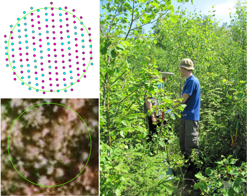
Fig. 2. An example of a seedling plot in ALS data, in aerial image with 25 cm resolution, and in the field. This plot needed tending immediately to free more growing space for the spruce seedlings. However, it is difficult to observe it from the ALS data (red dots are vegetation hits above 0.5 m, blue dots ground hits) or from the aerial image.
2.3 ALS and image features
Several height, density, intensity, spectral and textural features were extracted from the ALS data and aerial images, and used as predictors in the classification. All ALS features were computed separately for first and last echoes. The first step was to calculate the height distributions for each sample plot using AGL heights. All of the laser hits were included (i.e. no height threshold was applied). Weighted height percentiles 1, 5, 10, 20,…, 80, 90, 95, 99 (h1,…, h99) were computed, and the corresponding densities (p1,…, p99) were calculated for the respective percentiles. Height percentiles were calculated by summing the heights at AGL. For example, the metric h50 is the height at which 50% of the cumulative height has accumulated and p50 is the number of laser hits below h50 divided by all the laser hits on the plot. In addition, the mean and standard deviation of heights at AGL and the proportion of vegetation hits vs. ground hits using a threshold of 0.5 meters were calculated. Following intensity features were also computed: mean, standard deviation, and percentiles 10, 30, 50, 70, and 90.
Two types of features were calculated from the aerial images: textural and spectral. Textural features were calculated using pan-sharpened and orthorectified NIR bands. The image that captured the sample plot or grid cell closest to the nadir was always used. Firstly, grey-level co-occurrence matrices were constructed with 10 rescaling classes and a lag distance of five pixels as an average of all directions (0, 45, 90 and 135 degrees). A preliminary test was carried out in order to select these parameter values. Eleven textural metrics were then calculated as explained in Haralick et al. (1973). Spectral features were calculated by projecting the first echoes of ALS points to the original color and near-infrared bands (Level-2, no pan-sharpening) in the same manner as described in Packalén et al. (2009). The mean of the pixel values were fetched to each point by iterating through all images to which a point hit. Then the mean and standard deviation were calculated by plot from pointwise mean values. In addition, transformations NDVI = (NIR – RED)/(NIR + RED) and SR = NIR/RED were calculated from the mean values of the spectral bands.
2.4 Classification methods and accuracy assessment
2.4.1 Regression methods
Model for stem density was created first using linear regression. Only the dominant trees were considered, i.e. possible understory and overstory trees were ignored. The alternative models were evaluated based on their R2 and the absolute and relative root mean squared error.
As the tests indicated that classification should be based on just two classes (tending or no tending), logistic regression was tested as a parametric classifier. The R statistical software’s generalized linear model (glm) function was used to construct the models. Although the data had a hierarchical structure, normal models provided slightly better results than mixed models, because the variation within plots inside the stands was often considerable. If the hierarchical structure is stronger mixed models may provide better results.
Stepwise variable selection techniques were tested to find out candidate predictors, however, the final model selection was done by manual experimentation on different predictor combinations and transformations. As the models were also applied to a separate validation data set, only 3–5 predictors were accepted into a single logistic model to avoid over-fitting. Confusion matrices and kappa coefficient were calculated using leave-one-out cross validation (CV) and used to evaluate the alternative models. Overall accuracy (OA) is the percent of all observations classified correctly, producer’s accuracy is the percent of correct classifications in each class observed in the field, and user’s accuracy is the percent of correct classifications in each predicted class. The well-known Cohen’s kappa is calculated from a confusion matrix (Landis and Koch 1977). It is close to zero if the classification is no better than randomly selecting the class, and exactly one if the classification is perfect.
2.4.2 Support vector machine
Support vector machine (SVM) is a nonparametric classifier that has been successfully applied with remote sensing data, so we tested it as an alternative to the logistic modeling. Empirical evidence suggests that SVM classifiers are robust to high-dimensional data and noise and therefore suitable for remote sensing applications (Foody et al. 2004; Mountrakis et al. 2011).
The idea of the support vector machine classifier is to fit a separating hyperplane between two classes of data, so that the margin (minimum distance) between the class samples is maximized in the chosen feature space (Schölkopf and Smola 2002). Usually the chosen feature mapping of data samples to a feature space is non-linear and is implicitly performed by using some kernel function, so that the resulting feature space has a larger dimension than the original space of data. The utilization of a non-linear feature map allows the use of a separating hyperplane as a decision boundary in the feature space, so that this boundary can actually have a complex (non-linear) form in the original data space. Here, SVM classification was performed via an infinite dimensional feature map induced by radial Gaussian kernel with a free length-scale parameter (Schölkopf and Smola 2002). The length-scale parameter of the Gaussian kernel controls the properties of the feature map and is usually derived by using training data and cross validation.
Maximization of the margin between class samples in the feature space aims to find a separating hyperplane that also has good generalization properties for data samples that were not included in the training data (Schölkopf and Smola 2002). In many cases it is reasonable to assume that the data is not separable in the feature space and therefore it is useful to control the fit of the hyperplane by the use of some additional constraints. Here, the SVM classification was performed by using a ν-SVM (“nu-SVM”) algorithm, where parameter ν is used to control the properties of the hyperplane as explained in Schölkopf and Smola (2002).
The feature selection for the SVM was performed by using class label information (tending or no tending) for training data and a greedy forward feature selection (GFFS) approach as presented below (steps 1–3). During the feature selection process we used the CV technique for evaluating the features and also as a parameter optimization method for classifier.
Step 1 (Scaling of features): First, all the ALS and image features from the training and validation data sets were combined and scaled to range [0,1]. Although we used validation data features in feature scaling, it should be emphasized that the class label information of final validation data set was not used in any phase of the feature selection process.
Step 2 (GFFS with training data): The parameter ν of the SVM algorithm was fixed to 0.5. Based on this fixed value, Cohen’s kappa values were calculated for all the available features in training set (scaled according to Step 1) by using the leave-5-out CV evaluation. In each of these evaluations, the length-scale parameter of the Gaussian kernel was considered as a free parameter of the classifier and optimized via 10-fold CV (correspond to leave-21-out CV). The feature corresponding to the largest kappa value was chosen to be first in the set of selected features. The second feature was calculated by using again the Cohen’s kappa from the leave-5-out CV evaluation for concatenated two-component vectors, where the first component was the first selected feature and the second component was the feature in evaluation. All of the following features were selected in a similar manner, so that all of the previously selected features were concatenated with the selected feature and evaluated by using the Cohen’s kappa from the leave-5-out CV. We calculated ten features in total by using this approach.
Step 3 (Re-evaluation of GFFS features): We re-evaluated the selected set of ten features obtained via Step 2 by using subsets of features and the calculation of average kappa value of leave-k-out CV, using k = 1, k = 5 and k = 10. Based on the maximum average kappa value, the amount of selected features was reduced from ten to seven.
The evaluation of the ν-SVM classification for model data was based on leave-one-out CV and the seven selected features from the feature selection process. The evaluation of ν-SVM classification for the stand scale validation data was performed by using the classifier that was constructed by using the training data and the seven features from feature selection process. Hence the evaluation approaches for model and validation data were the same as in the case of logistic models. For the evaluation purposes, the classifier parameters (kernel length scale and ν) were optimized via 10-fold CV for the training data. Classification was calculated by using MATLAB 7.9 (The Mathworks, Inc.) and LIBSVM library (“nu-SVC”-classifier) by Chang and Lin (2011).
2.5 Calculation of the stand scale validation results
Tending need predictions are needed at stand level, so the separate stand scale validation data was used for final evaluation of the classifiers. Stand level predictions are not usually calculated directly for the stands, as the size of the prediction unit should be similar to the size of the modeling unit (sample plot) (Magnussen and Boudewyn 1998). Thus the study area was overlaid by a grid, and the predictor features were calculated for each grid cell similarly as for the training plots. Thus each stand consisted of several grid cells, each of which had its own predicted tending need (Fig. 3). The final stand level estimates were obtained by aggregating the grid cells that were within the stand borders. In Finnish practical RS inventories, the plot radius is usually nine meters, and thus the equivalent cell size in the application phase is 16 x 16 meters.
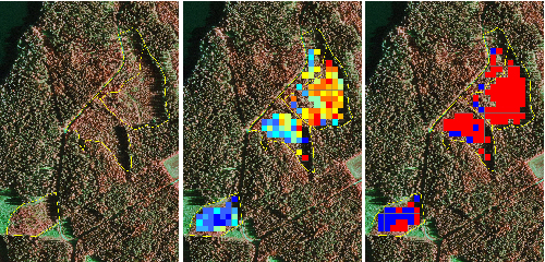
Fig. 3. Left: Four seedling stands delineated on an aerial image. Middle: Probability of tending need predicted by the logistic model. Right: Tending need predicted by the support vector machine. The red color indicates a need for tending and blue indicates no need. Note that some cells are missing because of the 10 meter height limit.
The stand level validation inventory was performed August-October 2011. A one year time lag between the data acquisition and the last field observations caused an additional source of error. We used the same remote sensing data from 2010 for training the models and validating them at stand level, but the prediction accuracy was evaluated one year after the data acquisition. Thus a stand that was in 2010 evaluated to need tending in the next year should be logically classified into the category “immediate” in 2011. There were also stands that had been tended between the scan and the inventory. In such cases we had to assume that the stand needed tending at the time of the scan, but its urgency could only be estimated from the stumps. However, the reclassification into only two classes (tending/no tending) helped to decrease these uncertainties.
The borders of the 80 stands in the validation data were obtained from a local database. The grid cells that had more than 90% of their intersection area inside the stand borders were selected to represent the stand. However, because the digitized stand borders did not always match the true borders, some cells could include trees from the neighboring stands.
It is a common practice to leave some retention trees and snags in the clearcut area to support biodiversity. When the training plots were placed into the stands, such trees were not allowed inside the plot radius, as the ALS height distribution should describe the seedling population and not the retention trees. Thus, also in the validation stands, the grid cells with echo heights larger than 10 m were left out of the analysis, as they either had retention trees or overlapped with a neighboring stand. The validation data also contained several stands that were at the edge of being classified as young forests instead of seedling stands (dominant height > 9 m). For 12 of these stands, the application of a 10 m height limit removed more than half of the original grid cells, and therefore the model could only be applied reliably to the remaining 68 stands. Thus the final validation data had 45 stands with an identified tending need and 23 stands with no need for tending (Table 2).
| Table 2. The number of stands by tree species and tending need class in the validation data. | ||||
| Tree species | Need for tending | Total | ||
| Immediately | 1–5 years | No need | ||
| Scots pine | 2 | 18 | 9 | 29 |
| Norway spruce | 7 | 14 | 13 | 34 |
| Deciduous trees | 3 | 1 | 1 | 5 |
| Total | 12 | 33 | 23 | 68 |
The stand-level predictions were aggregated from the individual cells by averaging the predicted values. For the logistic model, the averaged values were the probabilities of tending need in the cells. For the SVM, the predicted values were binary (tending or no tending), i.e. the stand scale result was similar to majority vote. Other aggregation options such as median and other threshold values than 0.5 were also tested to see if they were less sensitive to outlier cells, but no significant improvements were obtained this way.
We evaluated also how large the error rates would be if only a particular percentage of the stands with the most reliable predictions were left without field check. We evaluated the prediction uncertainty as Abs (stand mean prediction – 0.5), i.e. the closer the stand mean was to 0or 1, the larger was the reliability. Then we examined leaving out 25% (17/68) or 50% (34/68) of the stands that had the highest reliability, and calculated the overall accuracy and kappa only for these stands.
3 Results
3.1 Training data set
3.1.1 Prediction of stem density
The best linear model we found for the stem density is presented in Eq. 1:
![]()
where f_p70 is the 70% ALS first echo density percentile, f_h40 is the 40% ALS height percentile, and cont is the textural contrast calculated from the aerial images. The bias-corrected RMSE of this model was 2867 stems/ha (52.5%) and R2 = 0.50. The large absolute RMSE is partly explained by the very high stand densities in the area, which are caused by multi-stemmed deciduous trees such as willow and rowan, together with the birches that reproduce from the sucker shoots.
3.1.2 Classification into tending need classes
The features selected into the direct classification are displayed in Table 3 and the results obtained from leave-one-out CV in the modeling data are in Tables 3–5. The logistic model had three predictors, with overall accuracy = 77%, and kappa = 0.55. The SVM classifier performed better: using seven predictors, the respective values were 86% and 0.71. Notably the SVM result was obtained without aerial image features, but one ALS intensity feature was included together with four ALS height and two density percentiles. The logistic model had three predictors: ALS height and density features were supplemented by one image texture feature, the log-transformed sum average. The confusion matrices (Tables 4–5) show that the SVM was better at distinguishing plots where tending was needed, as ten more plots were correctly classified than with the logistic model.
| Table 3. The accuracies and predictive variables of the best models for tending need in the training data. Prefix f_ denotes first and l_ last echo. Savg is the “sum average” textural feature. | |||
| Model | Predictors | Overall accuracy | Kappa |
| Logit | f_h50, f_p40, log(savg) | 77% | 0.55 |
| SVM | l_h70, l_p40, l_p5, l_i50, f_h50, l_h30, l_h50 | 86% | 0.71 |
| Table 4. Confusion matrix of the tending need classification using the logistic model. OA = 77%, kappa = 0.55. | ||||
| Logistic model | Field value | |||
| Tending | No tending | Total | User’s accuracy | |
| Tending | 80 | 24 | 104 | 77% |
| No tending | 23 | 81 | 104 | 78% |
| Total | 103 | 105 | 208 | |
| Producer’s accuracy | 78% | 77% | ||
| Table 5. Confusion matrix of the tending need classification using the support vector machine. OA = 86%, kappa = 0.71. | ||||
| SVM | Field value | |||
| Tending | No tending | Total | User’s accuracy | |
| Tending | 90 | 17 | 107 | 84% |
| No tending | 13 | 88 | 101 | 87% |
| Total | 103 | 105 | 208 | |
| Producer’s accuracy | 87% | 84% | ||
Surprisingly, the spectral features were not used by any of the classifiers. High near-infrared reflectance should indicate deciduous species dominance, and most of the plots were located at stands that had pine or spruce as the preferred species. In order to confirm this we excluded the 27 plots that had birch as a main species and refitted the logistic models, but still the spectral features offered no improvement. The reason for this could be that most of the study area had fertile soils with a plentiful herbaceous vegetation that is spectrally similar to deciduous foliage. As the seedling stands usually have low canopy cover, the herbaceous understory was probably dominating the reflectance, even in the conifer stands.
| Table 6. Error rates in different stand parameter classes for the modeling and validation plots. Note that height was not estimated in the field for the validation stands, so ALS-based f_h80 was used instead*. | |||||||
| Model data | Validation data | ||||||
| n | Logistic error % | SVM error % | n | Logistic error % | SVM error % | ||
| Tending need | No need | 105 | 22.9 | 16.2 | 23 | 30.4 | 43.5 |
| 1–5 years | 66 | 28.8 | 18.2 | 33 | 36.3 | 21.2 | |
| Immediate | 37 | 10.8 | 2.7 | 12 | 8.3 | 16.7 | |
| Species | Pine | 104 | 26.0 | 14.4 | 29 | 41.4 | 37.9 |
| Spruce | 77 | 20.8 | 15.6 | 34 | 20.6 | 20.6 | |
| Deciduous | 27 | 14.8 | 11.1 | 5 | 20.0 | 20.0 | |
| Site type | Very fertile | 20 | 20.0 | 20.0 | 6 | 16.7 | 16.7 |
| Fertile | 134 | 20.9 | 14.9 | 53 | 28.3 | 30.2 | |
| Rather poor | 46 | 28.3 | 8.7 | 9 | 44.4 | 22.2 | |
| Poor | 8 | 25.0 | 25.0 | 0 | - | - | |
| Height (*f_h80) | 0–2 | 28 | 25.0 | 17.9 | 6 | 0.0 | 0.0 |
| 2–4 | 106 | 25.5 | 13.2 | 28 | 25.0 | 25.0 | |
| 4–6 | 57 | 19.3 | 17.5 | 29 | 37.9 | 34.5 | |
| 6+ | 17 | 11.8 | 5.9 | 5 | 40.0 | 40.0 | |
| Density | 0–2500 | 32 | 9.4 | 6.2 | 16 | 31.3 | 50.0 |
| 2500–5000 | 61 | 26.2 | 19.7 | 25 | 24.0 | 20.0 | |
| 5000–10000 | 66 | 33.3 | 21.2 | 23 | 34.8 | 26.1 | |
| >10000 | 49 | 12.2 | 4.1 | 4 | 25.0 | 0.0 | |
Although both logistic model and SVM performed reasonably well, the classification still retained plenty of errors (Table 6). It was difficult to find clear reasons for the misclassifications, as there were errors in all kinds of plots. However, both the logistic model and especially the SVM were quite accurate in stands with an immediate tending need and high stem density. Also the stands with low stem density were usually classified correctly, but in some cases the low density was not equivalent to a no tending recommendation. The deciduous stands were classified correctly more often than the conifer stands, especially with the logistic model. This could occur because in deciduous stands only the height and density are needed and the species composition has a smaller influence. In many cases where the models erroneously predicted tending, it was actually marked into data but only after the first five-year period. Contrastingly however, tending was often missed by the models in stands that had an uneven structure, for example when overstory trees have plenty of space yet there is fierce competition in the lowerstory.
3.2 Stand level validation data
When the area-based ALS inventory is applied to the stand level, the results are usually more accurate than in the plot level. This is because random errors cancel each other out when the predictions are averaged from the grid cells to the stand level. The stem density model indeed obtained slightly better accuracy in the stand level (RMSE = 2204 stems/ha or 49.7%). However, in the tending need classification the results were worse in the stand level (Tables 7–8). The OA and kappa were 71% and 0.38 for the logistic model. For the SVM classifier they were 72% and 0.37, respectively. Overall, the differences between the classifiers were small, but the logistic model was slightly better in recognizing stands without a tending need, whereas the SVM was better at recognizing stands that needed tending. Table 6 indicates that the stands with an immediate tending need and high density were again the easiest to classify correctly. The training data also suggested that stands with low density and deciduous dominance would be easier to classify correctly, but this was not the case in the validation data. However, in the validation data all the six stands with height = 0–2 m were correctly classified to have a tending need.
| Table 7. Confusion matrix of the logistic classifier in the validation stands. OA = 71%, kappa = 0.38. | ||||
| Logistic model | Field value | |||
| Tending | No tending | Total | User’s accuracy | |
| Tending | 32 | 7 | 39 | 82% |
| No tending | 13 | 16 | 29 | 55% |
| Total | 45 | 23 | 68 | |
| Producer’s accuracy | 71% | 70% | ||
| Table 8. Confusion matrix of the SVM classifier in the validation stands. OA = 72%, kappa = 0.37. | ||||
| SVM | Field value | |||
| Tending | No tending | Total | User’s accuracy | |
| Tending | 36 | 10 | 46 | 78% |
| No tending | 9 | 13 | 22 | 59% |
| Total | 45 | 23 | 68 | |
| Producer’s accuracy | 80% | 57% | ||
Almost 30% of the validation stands were classified incorrectly, which indicates that in our study area, the use of remote sensing cannot totally replace the field inventories. However, the RS-based interpretation is useful if it can classify even some of the stands reliably. The confusion matrices for leaving out 25% of the stands are displayed in Tables 9–10, and for leaving out 50%, in Tables 11–12. The results showed that the logistic model was very good at correctly recognizing the stands where the prediction was reliable: in the 25% case all of the selected stands were classified correctly, and in the 50% case, 91% of the stands were correct. However, the SVM results did not improve very significantly in this test (kappa = 0.40–0.43). The reliability of the SVM predictions is more difficult to assess, as a binary classifier does not have a clear probabilistic interpretation.
| Table 9. Confusion matrix of the logistic classifier for the omission of 25% of the validation stands having the highest reliability. OA = 100%, kappa = 1.00. | |||
| Logistic model | Field value | Total | |
| Tending | No tending | ||
| Tending | 14 | 0 | 14 |
| No tending | 0 | 3 | 3 |
| Total | 14 | 3 | 27 |
| Table 10. Confusion matrix of the SVM for the omission of 25% of the validation stands having the highest reliability. Overall accuracy = 81%, kappa = 0.43. | ||||
| SVM | Field value | |||
| Tending | No tending | Total | User’s accuracy | |
| Tending | 16 | 1 | 17 | 94% |
| No tending | 3 | 1 | 4 | 25% |
| Total | 19 | 2 | 21 | |
| Producer’s accuracy | 84% | 50% | ||
| Table 11. Confusion matrix of the logistic classifier for the omission of 50% of the validation stands having the highest reliability. Overall accuracy = 91%, kappa = 0.80. | ||||
| Logistic model | Field value | |||
| Tending | No tending | Total | User’s accuracy | |
| Tending | 21 | 0 | 21 | 100% |
| No tending | 3 | 10 | 13 | 77% |
| Total | 24 | 10 | 34 | |
| Producer’s accuracy | 88% | 100% | ||
| Table 12. Confusion matrix of the SVM for the omission of 50% of the validation stands having the highest reliability. Overall accuracy = 79%, kappa = 0.40. | ||||
| SVM | Field value | |||
| Tending | No tending | Total | User’s accuracy | |
| Tending | 23 | 3 | 26 | 88% |
| No tending | 4 | 4 | 8 | 50% |
| Total | 27 | 7 | 34 | |
| Producer’s accuracy | 85% | 57% | ||
The kappa and OA of the logistic model as a function of the percent of selected stands is illustrated in detail in Fig. 4. The first stand that was misclassified was 21st in the order of reliability, indicating that 30% of the stands could have been left without a field check so that no errors would have been made. All of the misclassified stands where the RS-based prediction appeared to be reliable were pine stands that had a tending need during the next 1–5 years, but moderate stem densities (4000–6000) and did not seem all that dense in the aerial images, so these errors should not be very drastic.
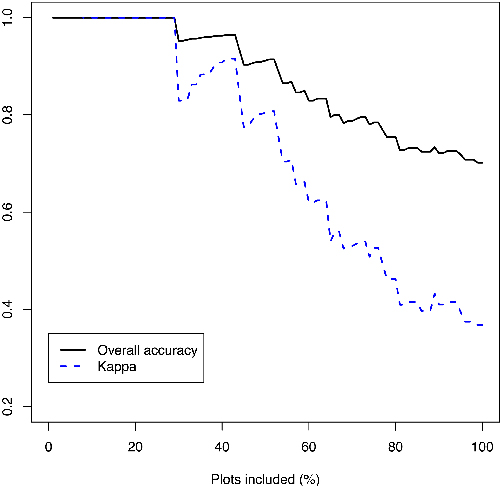
Fig. 4. Overall accuracy and kappa of the logistic model in the validation stands with the most reliable predictions. The percentage at the x-axis describes the proportion of stands that would be left without field check, and the y-axis shows the consequent model errors.
4 Discussion
The detection of different silvicultural needs with remote sensing is problematic since in practical forestry, such need is usually based on subjective field assessment. If the tending need is derived afterwards from field measurements of tree attributes, the results may be different. In the case of seedling stands, a different decision may be based on the reasons mentioned earlier in this study, i.e. a high number of small unimportant trees or perhaps long disturbing herbaceous vegetation. When this kind of classification situation is related to prediction by remote sensing material it is obvious that results with outstanding accuracy cannot be obtained. In this study, we had to simplify the classification problem from three to two classes, and still the overall accuracy was found to be only moderate.
Direct classification is however a better alternative than trying to estimate variables such as stem density, spatial pattern of seedlings, species proportions, height differences etc., all of which are evaluated when management decisions are made in the field. Our stem density RMSE = 49.7% is approximately twice as large as has been obtained in mature forests (Suvanto et al. 2005), and the species proportions would be even more difficult to estimate reliably. In this area the tending need could not be predicted reliably even by using the stem density measured in the field (Fig. 1). The use of field-measured stand attributes in predicting the tending need of spruce seedling stands was recently tested by Uotila et al. (2012). They used multinomial logistic models to classify the stands into three management need classes, and concluded that the measured stand characteristics were only useful for detecting the peripheral cases. However, they also found that some stable stand attributes such as soil dampness and treatment history could be used as additional predictors.
Although we were not able to achieve a very accurate classification of the whole validation data, the predicted probabilities obtained from a logistic regression model could be used to detect the stands for which the prediction was reliable. This is a very promising result and indicates that remote sensing can be used in the future to decrease the amount of field work required for seedling stands. Especially, the stands that were extremely dense and thus needed immediate tending were recognized fairly reliably using just three predictors – the ALS based height and density, and the image-based “sum average” describing the texture. An interesting observation was that in this study area, the ALS height percentiles had a strong negative correlation with the tending need, i.e. taller seedling stands were far less likely to need tending than younger ones. The stands with tall seedlings may of course need tending too, but on average, younger seedlings have a greater risk of being shadowed. Similarly, high ALS density (related to vegetation cover) had a positive correlation with the tending need, as well as a low heterogeneity quantified by the image texture. In some other regions the spectral features could also be useful predictors, but in this area they did not describe the proportion of deciduous species as well as in mature stands.
There are several important issues that need to be considered in practical seedling stand inventories. First, the training data set should be representative of all kinds of seedling stands occurring in the area, which may be difficult to achieve due to limited resources. In practical projects, the inventory area can be 1000–2000 km2, which is modeled using 500–700 sample plots. 100–150 of the plots are usually placed in seedling stands. Most of the seedling stands tend to be quite similar, so randomly selected plot locations may not cover the entire scale of ALS and aerial image features that were selected for the models. Thus stratification is needed. Due to out-of-date stand registers our field crew had to spend plenty of time searching for stand types that were not yet well enough represented in the training data. This might not always be possible due to limited resources, and therefore our seedling data set was probably better than can be assumed in practical inventories. Solving this issue would require that the RS data used for modeling would be available already in the plot selection phase, which is difficult as the field work and RS data acquisition should be ideally performed at the same time.
Secondly, the quality of field-based tending need estimates must be confirmed. Our field work was initially done by two forestry students, who were sometimes unsure about the correct treatment of the stand. Thus we asked a local professional to double-evaluate the tending need, and the results showed that the estimates made by the professional were more consistent and hence easier to model than that of the students. In practice, field measurements are often performed by short-term workers, meaning that they must be trained very well in order to reliably estimate the tending need.
The comparison of the two classification methods indicated that parametric methods such as logistic regression can provide acceptable predictions. The SVM classifier was better fitted to the training data, but in the separate stand level validation data, the differences to the logistic model disappeared. The advantage of the logistic model was the probabilistic interpretation of the predictions, which assisted the detection of stands where the certainty of the predictions was high. Other than this, the results indicate that the selection of the predictor features has much larger influence than the selection of the classifier. Height and density features calculated from the ALS data describe the geometry of the seedling stand and thus the competition between the seedlings, and form the basis for the classification. However, if the aerial images have higher resolution than the ALS data (as was the case in our data), the image texture features may provide additional information. In some cases also the spectral features may be useful as they potentially describe the species proportions, but we did not see this effect in our data. We also noticed that as we gradually identified errors in the training data set and removed them, the previously selected features did not provide the best results any more, i.e. the variable selection was sensitive to small changes in the modeling data. This observation also emphasizes the importance of obtaining a representative and consistently estimated base data that does not contain errors.
Finally, when the models are applied to predict the tending needs for stands, the selection of the grid cells that are used in making the predictions is crucial. The existing stand borders may contain errors, meaning that some of the grid cells from which the stand level predictions were averaged, could partly belong to a neighboring stand. Also the presence of retention trees distorts the ALS height distributions for some of the cells. The results improved significantly when we applied a ten meter height limit for the cells accepted for prediction, which removed both border cells that did not belong to the stand in question and those cells with retention trees.
Although the analysis of seedling stands from remotely sensed data is a difficult task and some field work is still needed, the ALS-based tending need predictions are still of use in practical forestry. These predictions should be combined with existing stand register data (such as site fertility, age and species) and local knowledge. If the model prediction is clear for a particular stand and other available information supports it, then the cost of checking tending needs in the field may be larger than the cost of possible errors. The methods developed in this study are already used in stand level forest management inventories in Finland, and the experiences regarding their suitability in practice are collected from across the country. However, further development and a facility that enables the adjustment to local conditions and user requirements will need to be undertaken by the service providers that deliver RS-based inventory products to the end-users.
5 Conclusion
The stem density models were relatively inaccurate as expected, and even the field-measured density was not explicitly related to tending need. Thus direct classification of stands into tending need classes should be preferred, although the prediction accuracy in the validation data was only moderate (kappa = 0.37–0.38 for two classes). The models were based on ALS features and aerial image texture; spectral information did not improve the models in this case. The stands that had very high stem density and needed tending immediately were the easiest to classify correctly. Parametric logistic regression and nonparametric SVM classifiers produced equally good overall classification in the validation stands, but the logistic model was better at identifying the stands where the predictions were reliable as it has a clear probabilistic interpretation. Up to 30% of the considered stands could have been left without a field check so that no errors would have been made.
Acknowledgements
We are thankful to Heikki Eronen, Jukka Hoppula and Teemu Saramäki for performing most of the field work, and the reviewers for their useful feedback. This research was supported by the Ministry of Agriculture and Forestry (research project “MMM Taimikkolaser”) and the strategic funds from the University of Eastern Finland.
References
Chang C.-C., Lin C.-J. (2011). LIBSVM : a library for support vector machines. ACM Transactions on Intelligent Systems and Technology 2: 27:1–27:27.
Foody G.M., Mathur A. (2004). A relative evaluation of multiclass image classification by support vector machines. IEEE Transactions on Geoscience and Remote Sensing 42(6): 1335–1343.
Hall R.J., Aldred A.H. (1992). Forest regeneration appraisal with large-scale aerial photographs. Forestry Chronicle 68(1): 142–150.
Haralick R.M., Shanmugam K., Dinstein I. (1973). Textural features for image classification. IEEE Transactions on Systems, Man and Cybernetics 3(6): 610–621.
Huuskonen S., Hynynen J. (2006). Timing and intensity of precommercial thinning and their effects on the first commercial thinning in Scots pine stands. Silva Fennica 40(4): 645–662.
Hyvönen P. (2002). Kuvioittaisten puustotunnusten ja toimenpide-ehdotusten estimointi k-lähimmän naapurin menetelmällä Landsat TM -satelliittikuvan, vanhan inventointitiedon ja kuviotason tukiaineiston avulla. [Estimation of stand attributes and management operations using Landsat TM satellite imagery, old inventory data and additional stand-level data]. Metsätieteen aikakauskirja 2002(3): 363–379. [In Finnish].
Korpela I., Tuomola T., Tokola T., Dahlin B. (2008). Appraisal of seedling-stand vegetation with airborne imagery and discrete-return LiDAR – an exploratory analysis. Silva Fennica 42(5): 753–772.
Korpela I.,Ørka H.O., Hyyppä J., Heikkinen V., Tokola T. (2010). Range and AGC normalization in airborne discrete-return LiDAR intensity data for forest canopies. ISPRS Journal of Photogrammetry and Remote Sensing 65(4): 369–379.
Magnussen S., Boudewyn P. (1998). Derivations of stand heights from airborne laser scanner data with canopy-based quantile estimation. Canadian Journal of Forest Research 28(7): 1016–1031.
Maltamo M., Packalén P., Kallio E., Kangas J., Uuttera J., Heikkilä J. (2011). Airborne laser scanning based stand level management inventory in Finland. Proceedings of Silvilaser 2011, Hobart, Australia. 10 p.
Mountrakis G., Im J., Ogole C. (2011). Support vector machines in remote sensing: a review. ISPRS Journal of Photogrammetry and Remote Sensing 66(3): 247–259.
Landis R.J., Koch G.G. (1977). The measurement of observer agreement for categorical data. Biometrics 33: 159–174.
Närhi M., Maltamo M., Packalén P., Peltola H., Soimasuo J. (2008). Kuusen taimikoiden inventointi ja taimikonhoidon kiireellisyyden määrittäminen laserkeilauksen ja metsäsuunnitelmatiedon avulla. [Inventory of spruce seedling stands and determination of tending need by means of laser scanning and forestry plan information]. Metsätieteen aikakauskirja 2008(1): 5–15. [In Finnish].
Næsset E. (2002). Predicting forest stand characteristics with airborne scanning laser using a practical two-stage procedure and field data. Remote Sensing of Environment 80(1): 88–99.
Næsset E., Bjerknes K.-O. (2001). Estimating tree heights and number of stems in young forest stands using airborne laser scanner data. Remote Sensing of Environment 78(3): 328–340.
Nivala M. (2012). Laserkeilauksen käyttö metsänhoitotarpeen määrittämisessä taimikoissa ja nuorissa kasvatusmetsiköissä. Summary: Using Laser scanning to examine need for forest management in seedlings and young forest stands. M.Sc. thesis. University of Eastern Finland. 65 p. [In Finnish].
Packalén P., Maltamo M. (2007). The k-MSN method for the prediction of species-specific stand attributes using airborne laser scanning and aerial photographs. Remote Sensing of Environment 109(3): 328–341.
Packalén P., Suvanto A., Maltamo M. (2009). A two stage method to estimate species-specific growing stock by combining ALS data and aerial photographs of known orientation parameters. Photogrammetric Engineering and Remote Sensing 75(12): 1451–1460.
Pesonen A., Korhonen K.T., Tuominen S., Maltamo M., Lukkarinen E. (2007). Taimikonhoitotarpeen arviointi valtakunnan metsien inventoinnin metsävarakartan pohjalta. [Assessment of seedling stand tending need based on national forest inventory forest resource maps]. Metsätieteen aikakauskirja 2007(2): 77–86. [In Finnish].
Pippuri I., Kallio E., Maltamo M., Peltola H., Packalén P. (2012). Exploring horizontal area-based metrics to discriminate the spatial pattern of trees and need for first thinning using airborne laser scanning. Forestry 85(2): 305–314.
Pouliot D.A., King D.J., Pitt D.G. (2002). Automated assessment of hardwood and shrub competition in regenerating forests using leaf-off airborne imagery. Remote Sensing of Environment 102(3–4): 223–236.
Schölkopf B., Smola A.J. (2002). Learning with kernels. Cambridge, MA, MIT Press.
Suvanto A., Maltamo M., Packalén P., Kangas J. (2005). Kuviokohtaisten puustotunnusten ennustaminen laserkeilauksella. [Prediction of stand attributes with airborne laser scanning]. Metsätieteen aikakauskirja 2005(4): 413–428. [In Finnish].
Tahvanainen K. (2011). Taimikonhoitotarpeen kartoitus laserkeilausaineiston, laserkeilausaineistosta ennustettujen puustotietojen ja taimikon perustamisilmoitusten avulla. [Prediction of seedling stand management need using laser scanning, stand attributes predicted with laser scanning, and seedling stand establishment notifications]. M.Sc. thesis. University of Eastern Finland. 43 p. [In Finnish].
Tapio. (2006). Hyvän metsänhoidon suositukset. [Recommendations for forest management in Finland]. Forest Development Centre Tapio. Metsäkustannus oy. 100 p. [In Finnish].
Tuomola T., Hämäläinen J., Räsänen T. (2006). Numeeriset ilmakuvat taimikon perkaustarpeen määrittämisessä. Summary: Use of digital aerial photographs in specifying the need for pre-commercial thinning. Metsätehon katsaus 24. 4 p. [In Finnish].
Uotila K., Rantala J., Saksa T. (2011). Kustannustehokas ja kannattava metsänuudistamisketju. [Cost-efficient and profitable forest regeneration chain]. Metsätieteen aikakauskirja 2011(1): 35–38. [In Finnish].
Uotila K., Rantala J., Saksa T. (2012). Estimating the need for early cleaning in Norway spruce plantations in Finland. Silva Fennica 46(5): 683–693.
Vastaranta M., Holopainen M., Yu X., Hyyppä H., Viitala R. (2011). Predicting stand-thinning maturity from airborne laser scanning data. Scandinavian Journal of Forest Research 26(2): 187–196.
Total of 29 references
