Jouni Siipilehto  ,
Micky Allen,
Urban Nilsson,
Andreas Brunner,
Saija Huuskonen,
Soili Haikarainen,
Narayanan Subramanian,
Clara Antón-Fernández,
Emma Holmström,
Kjell Andreassen,
Jari Hynynen
,
Micky Allen,
Urban Nilsson,
Andreas Brunner,
Saija Huuskonen,
Soili Haikarainen,
Narayanan Subramanian,
Clara Antón-Fernández,
Emma Holmström,
Kjell Andreassen,
Jari Hynynen
Stand-level mortality models for Nordic boreal forests
Siipilehto J., Allen M., Nilsson U., Brunner A., Huuskonen S., Haikarainen S., Subramanian N., Antón-Fernández C., Holmström E., Andreassen K., Hynynen J. (2020). Stand-level mortality models for Nordic boreal forests. Silva Fennica vol. 54 no. 5 article id 10414. https://doi.org/10.14214/sf.10414
Highlights
- Models were developed for predicting stand-level mortality from a large representative NFI data set
- The logistic function was used for modelling the probability of no mortality and the proportion of basal area in surviving trees
- The models take into account the variation in prediction period length and in plot size
- The models showed good fit with respect to stand density, developmental stage and species structure, and showed satisfying fit in the independent data set of unmanaged spruce stands.
Abstract
New mortality models were developed for the purpose of improving long-term growth and yield simulations in Finland, Norway, and Sweden and were based on permanent national forest inventory plots from Sweden and Norway. Mortality was modelled in two steps. The first model predicts the probability of survival, while the second model predicts the proportion of basal area in surviving trees for plots where mortality has occurred. In both models, the logistic function was used. The models incorporate the variation in prediction period length and in plot size. Validation of both models indicated unbiased mortality rates with respect to various stand characteristics such as stand density, average tree diameter, stand age, and the proportion of different tree species, Scots pine (Pinus sylvestris L.), Norway spruce (Picea abies (L.) Karst.), and broadleaves. When testing against an independent dataset of unmanaged spruce-dominated stands in Finland, the models provided unbiased prediction with respect to stand age.
Keywords
Norway spruce;
Scots pine;
simulation;
broadleaved species;
logistic function;
period length;
plot size
-
Siipilehto,
Natural Resources Institute Finland (Luke), Natural resources, P.O. Box 2, FI-00790 Helsinki, Finland
E-mail
jouni.siipilehto@luke.fi
-
Allen,
Norwegian Institute of Bioeconomy Research (NIBIO), Division of Forest and Forest Products, NO-1431 Ås, Norway; Larson and McGowin Inc., Mobile, AL 36607, USA
 https://orcid.org/0000-0002-7824-2849
E-mail
micky.allen@nibio.no
https://orcid.org/0000-0002-7824-2849
E-mail
micky.allen@nibio.no
-
Nilsson,
Swedish University of Agricultural Sciences (SLU), Southern Swedish Forest Research Centre, SE-23053 Alnarp, Sweden
https://orcid.org/0000-0002-7624-4031
E-mail
urban.nilsson@slu.se
-
Brunner,
Norwegian University of Life Sciences (NMBU), Faculty of Environmental Sciences and Natural Resource Management, NO-1432 Ås, Norway
https://orcid.org/0000-0003-1668-9714
E-mail
andreas.brunner@nmbu.no
-
Huuskonen,
Natural Resources Institute Finland (Luke), Natural resources, P.O. Box 2, FI-00790 Helsinki, Finland
https://orcid.org/0000-0001-8630-3982
E-mail
saija.huuskonen@luke.fi
-
Haikarainen,
Natural Resources Institute Finland (Luke), Natural resources, P.O. Box 2, FI-00790 Helsinki, Finland
https://orcid.org/0000-0001-8703-3689
E-mail
soili.haikarainen@luke.fi
-
Subramanian,
Swedish University of Agricultural Sciences (SLU), Southern Swedish Forest Research Centre, SE-23053 Alnarp, Sweden
https://orcid.org/0000-0003-2777-3241
E-mail
narayanan.subramanian@slu.se
-
Antón-Fernández,
Norwegian Institute of Bioeconomy Research (NIBIO), Division of Forest and Forest Products, NO-1431 Ås, Norway
https://orcid.org/0000-0001-5545-3320
E-mail
clara.anton.fernandez@nibio.no
-
Holmström,
Swedish University of Agricultural Sciences (SLU), Southern Swedish Forest Research Centre, SE-23053 Alnarp, Sweden
https://orcid.org/0000-0003-2025-1942
E-mail
emma.holmstrom@slu.se
-
Andreassen,
Norwegian Institute of Bioeconomy Research (NIBIO), Division of Forest and Forest Products, NO-1431 Ås, Norway
https://orcid.org/0000-0003-4272-3744
E-mail
kjellandreassen@gmail.com
- Hynynen, Natural Resources Institute Finland (Luke), Natural resources, P.O. Box 2, FI-00790 Helsinki, Finland E-mail jari.hynynen@luke.fi
Received 7 July 2020 Accepted 24 November 2020 Published 1 December 2020
Views 102358
Available at https://doi.org/10.14214/sf.10414 | Download PDF

1 Introduction
Sustainable use of forest resources requires reliable information both on the current state of forests, and forecasts on the development of forest resources under changing environment and alternative management strategies (Buongiorno and Gilless 2003; Keenan 2015). Trustworthy estimates of the long-term development of forests rely on the thoroughgoing knowledge of the structure and dynamic of forests at the stand-level, including the impacts of the different abiotic and biotic factors as well as the effects of silvicultural treatments on stand development (Fortin et al. 2008; Sims et al. 2014). Wide varieties of stand structures, management histories, and growth environments set a high demand for models predicting stand dynamics, which are designed to be applied in decision support tools for forest management planning. Empirical data used in modelling and model validation should cover the same range of variation in crucial factors affecting forest dynamics. Besides comprehensive modelling data, the structure of models should provide a logical behavior when applied outside the range of modelling data.
In addition to stand growth, an understanding of tree mortality, caused by the natural ageing of the trees, competition between the trees, and/or abiotic or biotic damage, is important to accurately predict forest dynamics (Taylor et al. 2009; Bircher et al. 2015). Mortality is one of the least predictable components of growth and yield estimation (Hamilton 1986; Fortin et al. 2008; Sims et al. 2014; Salas-Eljatib and Weiskittel 2020). Mortality is often divided into regular competition-related mortality and more irregular catastrophic mortality (Vanclay 1994). Yli-Kojola (2005), Laarmann et al. (2009), and Sims et al. (2014) have found that competition was the most common reason for tree mortality in Finland and in Estonia. In general, trees with relatively low diameter were more likely to die because of tree competition whereas increasing relative tree size increased the likelihood of insect and wind damage (Yli-Kojola 2005; Laarmann et al. 2009; Sims et al. 2014; Yao et al. 2001; Vieilledent et al. 2009). Quite often the main cause of mortality remained unknown (Yli-Kojola 2005; Laarmann et al. 2009).
The most common function used to model the probability of tree-level mortality is the logistic function. Individual tree mortality can be predicted from variables such as tree growth, crown and stem dimensions, dominance, and competition in addition to some stand, site and environmental variables (Salas-Eljatib and Weiskittel 2020). In a single tree-based stand simulator stand-level mortality is the outcome from tree-level mortality (Fortin et al. 2008). Stand-level models are often preferred over tree-level models because they are less data intensive with regard to model development and application inputs (Affleck 2006; Weiskittel et al. 2011). In general, stand-level mortality models are developed in two-steps, the first step being prediction of the probability of mortality and the second step prediction of the amount of mortality (Woollons 1998; Fridman and Ståhl 2001; Eid and Øyen 2003; Álvarez et al. 2004). The amount of mortality is traditionally modelled as a reduction in stem number (Woollons 1998; Eid and Øyen 2003; Álvarez et al. 2004). However, Fridman and Ståhl (2001) presented a model for the predicting the amount of mortality as a proportion of the initial basal area.
So far, each of the Nordic countries have independently developed their own model-based forest management planning and simulation tools, which include stand- and tree-level models for forest dynamics, i.e. Mela (Siitonen 1995; Siitonen and Nuutinen 1996) and Motti (Salminen et al. 2005) in Finland, Hugin (Lundström and Söderberg 1996) and Heureka (Lämås and Eriksson 2003; Wikström et al. 2011; Fahlvik et al. 2014) in Sweden, and AVVIRK-2000 (Eid and Hobbelstad 2000), GAYA-JLP (Hoen and Eid 1990) and SiTree (Antón-Fernández et al. 2019) in Norway. In all Nordic countries, the mortality models applied in planning tools are based either on national forest inventory (NFI) data from permanent sample plots (Fridman and Ståhl 2001; Eid and Tuhus 2001), or inventory growth plot data being a subsample of NFI plots (Hynynen et al. 2001). All the previously mentioned Nordic models included both regular mortality due to competition and mortality from irregular hazards (snow, wind), if they have occurred.
The aim of this study was to provide reliable stand-level mortality models which also enable long term growth and yield simulations and thus provide information of carbon stock development in old forest stands. The general purpose of this study was to improve the predictions for stand-level mortality in decision support tools applied in Finland, Norway, and Sweden. Given similar forest types, mortality models based on combined data from Sweden and Norway can also be applied in forest development simulations in Finland. Combining data for the region also increased the variation in management regimes and the amount of data from mature and old stands, which are scarce in each country, but essential for the simulation of extended rotation times. More precisely, the aim was to construct stand-level mortality models for stands dominated by Scots pine (Pinus sylvestris L.) and Norway spruce (Picea abies (L.) Karst.)(hereafter referred as pine and spruce), which perform reliably for mature stands and for stands which have exceeded the commercial rotation age and also take into account the effects of tree species composition on mortality rates.
2 Material and methods
2.1 Overview of modelling approach
Data from permanent NFI plots in Norway and Sweden were used for developing the new mortality models. NFI data are a representative sample of forest areas, describing the structure and dynamics of current forest stands (Fridman et al. 2014; Tuominen et al. 2014). This study proceeded via two steps. First, available data in Norway and Sweden were examined and a common database was constructed. In the second step, stand-level mortality models were constructed and evaluated. In the model development stage, a stand-level modelling approach was applied for predicting i) probability of no mortality occurrence in a stand, and when mortality occurs ii) survival in terms of basal area of surviving trees relative to total basal area. Logistic regression models were constructed for both cases because the logistic equation ensured a logical model behavior due to the range of possible values between zero and one (Hosmer and Lemeshow 1989). The new models were then examined within the Motti simulator using an independent data set from Finland.
2.2 Modelling data sets
Initially, NFI data from each country were considered. However, during the early phase of the data analysis, the structure of the Finnish data was found to differ significantly from the NFIs of Sweden and Norway. Permanent sample plots in Finland (INKA) were established only in stands in which stand structure was more homogeneous than on the average. Therefore, only the NFI data from Sweden and Norway were used for model fitting.
The Swedish NFI data used for modelling was a subsample of the permanent NFI plots with area of 314 m2. The permanent sample plots were established 1983–1987 with a re-sampling frequency of mostly five years (Fridman et al. 2014). On each permanent plot, all trees above 10 cm dbh were measured and ingrowth trees were included once reaching 10 cm. Missing trees with located stumps were registered as harvested and dead standing or fallen trees remained on site were registered as dead. All registered trees were cross-calipered at breast height (1.3 m).
The Norwegian NFI data consist of a series of permanent sample plots established during the period 1986–1993 (Tomter et al. 2010). The plots are located at the intersections of a 3×3 km grid except for areas which are above the coniferous tree line or in the northernmost county of Finnmark where wider grids of 3×9 km or 9×9 km are used, respectively. Each plot is measured every 5-years. All trees above 5 cm dbh were measured. At first, the permanent plot size was 100 m2 (Eid and Tuhus 2001), but plot size was enlarged to 250 m2 since 1994 (Tomter et al. 2010).
For modelling, a uniform structure of the pooled data set was needed. Therefore, all the initial NFI-plots were not included to the modelling data set and some modifications were needed when converting data from different countries into a common format. For the mortality models, all sample plots with land use class of “forest land” were included. In the Swedish data, the plot size was a constant 314 m2 (radius 10 m) while in the Norwegian data, only plots of 250 m2 (radius 8.9 m) were used. Finally, to be uniform to the Swedish NFI data, only trees with a breast height diameter of at least 10 cm were included.
The following restrictions were also set for the data during the modelling process. The minimum temperature sum was set for 300 degree days (ddy), excluding harsh growing conditions. Minimum stand age was set to 10 years and minimum stand mean diameter was set for 15 cm. Finally, minimum stem number was set for 80 trees ha–1, meaning that at least three sample trees were measured in each NFI plot. The oldest measurement occasions (i.e., years earlier than 2000) were excluded, because knowledge of the harvests was not available in Norwegian data set until year 2000.
The model fitting data set included sample plots located on both mineral soil and peatland soil sites. In the Swedish data, soil moisture was re-coded from five classes to the three classes used in Norway (i.e., initial Swedish class 1 = moisture class 1 (dry), initial Swedish class 2 or 3 = moisture class 2, initial Swedish class 4 or 5 = moisture class 3 (moist)). Finally, from these three classes two categorical variables were produced for modelling, dummy variables for dry (class 1) and moist (class 3) site. The temperature sums (DDY) common for each country were based on the 5 °C threshold, plot coordinates and altitudes and represented long-term averages from 1981 to 2010. For each NFI plot in the combined data set, the main tree species was defined according to the tree species with the largest proportion of basal area on the plot. The number of measurements for each NFI plot varied from two to five, and thus, the measurement periods from one to four. The time between two measurements (period) was calculated from the initial measurement dates included in each data sets. The most common growing period was 5 years but varied from 4 to 6 years.
Stand characteristics (number of trees, basal area, and mean diameter) were similarly calculated from trees larger than or equal to 10 cm in both data sets. Characteristics were calculated separately for living, dead, and harvested trees and by tree species groups (pine, spruce, broadleaved species, e.g. birch (Betula pendula Roth and B. pubescens Ehrh.), aspen (Populus tremula L.) and alder (Alnus incana L. and A. glutinosa (L.) Gaertn.). Stand age refers to the average total age of the growing stock. Information on stand height varied between countries and therefore height variables were not used in modelling. Similarly, the site index calculated in each country was derived differently and was not used for model fitting.
Variables and their definitions are summarized in Table 1. The final set of the Swedish NFI data for modelling included 6860 plots, and 16 459 observations. Accordingly, the final set of the Norwegian NFI data for modelling included 6046 plots, and 11 767 observations (Table 2). For fitting the first model, which predicts the probability of no mortality, the total combined data set (Table 2) was used. For fitting the second model, which predicts the proportion of basal area in surviving trees, only the plots where dead trees were registered between adjacent measurements were used. The number of observations for fitting the second model was 4218 in Sweden and 3107 in Norway from the total number of 7325 observations (Table 3).
| Table 1. Variables for the models, their symbols, and units. | ||
| Variable | Symbol | Unit |
| Plot size | Plotsize | m2 |
| Cumulative annual daily mean temperatures above +5 °C | DDY | degree days (d.d.) |
| Height above sea level | Altitude | m |
| Slope | Slope | % |
| Latitude | Latitude | min |
| Mean total age of stand | Age | years |
| Number of stems | N | N ha–1 |
| Basal area | BA | m2 ha–1 |
| Mean diameter, basal area weighted | DG | cm |
| Basal area of pine trees | BApine | m2 ha–1 |
| Basal area of spruce trees | BAspruce | m2 ha–1 |
| Basal area of broadleaved trees | BAbrd | m2 ha–1 |
| Proportion of pine basal area of total basal area | BApineRel | |
| Proportion of broadleaved basal area of total basal area | BAbrdRel | |
| Number of dead tree stems | N_dead | N ha–1 |
| Basal area of dead trees | BA_dead | m2 ha–1 |
| Mean diameter of dead trees, basal area weighted | DG_dead | cm |
| Occurence of mortality | mortality | {0, 1} |
| Soil type peatland | PEAT | {0, 1} |
| Aspect between 225 and 315 degrees, when max was 360 | WEST | {0, 1} |
| Growth period between measurements | Period | years |
| Thinning within 5 years of the studied period | TH5 | {0, 1} |
| Quadratic mean diameter, √(BA/qN) | DQ | cm |
| Occurrence of mortality: 0 = mortality occur; 1 = no mortality occur; Peatland: 0 = no peatland, 1 = peatland; Western aspect: 0 = no western aspect, 1 = western aspect; Thinning within 5 yrs: 0 = not thinned, 1 = thinned | ||
| Table 2. Description of combined Swedish and Norwegian NFI data for modelling the occurrence of no mortality. | ||||||
| Data set | SWEDEN (n = 16 459 ) | NORWAY (n = 11 767) | ||||
| Variable | mean | min | max | mean | min | max |
| Plotsize, m2 | 314.2 | 314.2 | 314.2 | 250.0 | 250.0 | 250.0 |
| DDY, d.d. | 1133.6 | 426.8 | 1760.4 | 881.1 | 303.5 | 2049.3 |
| Altitude, m | 228.7 | 0.0 | 787.0 | 379.4 | 0.0 | 1080.0 |
| Slope, % | 4.8 | 0.0 | 41.5 | 25.0 | 0.0 | 150.0 |
| Latitude, min | 6104.0 | 5540.0 | 6830.0 | 6156.8 | 5800.5 | 7001.4 |
| Age, yr | 80.6 | 11.0 | 325.0 | 102.6 | 19.0 | 374.0 |
| N, ha–1 | 685.8 | 95.5 | 2387.3 | 579.1 | 120.0 | 2560.0 |
| BA, m2 ha–1 | 21.7 | 1.4 | 73.0 | 17.5 | 1.8 | 113.2 |
| DG, cm | 23.6 | 15.0 | 93.7 | 23.3 | 15.0 | 71.2 |
| BApine, m2 ha–1 | 9.2 | 0.0 | 60.1 | 6.3 | 0.0 | 57.2 |
| BAspruce, m2 ha–1 | 9.1 | 0.0 | 73.0 | 7.4 | 0.0 | 113.2 |
| BAbrd, m2 ha–1 | 3.4 | 0.0 | 60.6 | 3.8 | 0.0 | 53.4 |
| BApineRel | 0.5 | 0.0 | 1.0 | 0.4 | 0.0 | 1.0 |
| BAbrdRel | 0.2 | 0.0 | 1.0 | 0.3 | 0.0 | 1.0 |
| N_dead, ha–1 | 13.5 | 0.0 | 954.9 | 17.2 | 0.0 | 680.0 |
| BA_dead, m2 ha–1 | 0.376 | 0.0 | 44.3 | 0.391 | 0.0 | 25.8 |
| DG_dead, cm | 17.8 | 10.0 | 75.8 | 16.4 | 10.0 | 58.9 |
| mortality, {0, 1} | 0.3 | 0.0 | 1.0 | 0.3 | 0.0 | 1.0 |
| Table 3. Description of sub data, which contained mortality at the following period, for modelling the amount of mortality. | ||||||
| Data set | SWEDEN (n = 4218) | NORWAY (n = 3107) | ||||
| Variable | mean | min | max | mean | min | max |
| DDY, d.d. | 1141.2 | 426.8 | 1732.9 | 890.4 | 303.5 | 1873.1 |
| Altitude, m | 226.8 | 0.0 | 761.0 | 354.1 | 2.0 | 1015.0 |
| Slope, % | 5.0 | 0.0 | 33.1 | 28.8 | 0.0 | 130.0 |
| Latitude, min | 6096.2 | 5540.0 | 6800.0 | 6172.1 | 5800.5 | 7001.4 |
| Age, yr | 84.1 | 11.0 | 325.0 | 100.5 | 19.0 | 318.0 |
| N, ha–1 | 826.4 | 95.5 | 2387.3 | 748.9 | 120.0 | 2560.0 |
| BA, m2 ha–1 | 25.2 | 2.1 | 61.9 | 22.2 | 1.8 | 113.2 |
| DG, cm | 23.3 | 15.0 | 71.0 | 23.1 | 15.0 | 56.6 |
| BApine, m2 ha–1 | 9.1 | 0.0 | 51.1 | 5.0 | 0.0 | 54.6 |
| BAspruce, m2 ha–1 | 11.4 | 0.0 | 58.6 | 10.8 | 0.0 | 113.2 |
| BAbrd, m2 ha–1 | 4.7 | 0.0 | 54.9 | 6.3 | 0.0 | 53.4 |
| BApineRel | 0.38 | 0.00 | 1.00 | 0.24 | 0.00 | 1.00 |
| BAbrdRel | 0.20 | 0.00 | 1.00 | 0.36 | 0.00 | 1.00 |
| N_dead, ha–1 | 52.7 | 31.8 | 954.9 | 65.1 | 40.0 | 680.0 |
| BA_dead, m2 ha–1 | 1.5 | 0.3 | 44.3 | 1.5 | 0.3 | 25.8 |
| DG_dead, cm | 17.8 | 10.0 | 75.8 | 16.4 | 10.0 | 58.9 |
| BArelMort | 0.062 | 0.050 | 0.986 | 0.083 | 0.050 | 0.970 |
2.3 Data set for model application
The data for demonstrating model application consisted of 57 plots of unmanaged spruce-dominated stands in Finland. The study plots were established between 1991 and 1999 in stands that had remained unmanaged (Isomäki et al. 1998). A few indications of past selective cutting were still found and thus, the stands are considered nearly natural forests (Peltoniemi and Mäkipää 2011). Typical plot sizes were 2500 m2 and 900 m2. Sites were mainly mesic heathlands but some grove like sites were also present, with the proportion of spruce ranging from 52–100% by basal area. The stands were located from Ostrobothnia (DDY 928 d.d.) to southern Finland (DDY 1411 d.d.). Initial stand ages varied from 80 to 290 yrs (Table 4). The youngest stands were most likely naturally regenerated after large-scale natural disturbances (Peltoniemi and Mäkipää 2011). The average basal area of dead trees (trees that died within measurement period) represented 9.6% of the initial stand basal area (Table 4). A large difference between the two mean diameters, quadratic mean diameter DQ and basal area weighted mean diameter DG, indicated wide and skewed diameter distributions which could be seen in Peltoniemi and Mäkipää (2011). The period length between the two measurements varied from 7 to 15 yrs. A description of this data set is presented in detail by Peltoniemi and Mäkipää (2011).
| Table 4. Description of the model application data, which contained 57 unmanaged spruce-dominated plots in Finland (see Peltoniemi and Mäkipää 2011). | ||||||||||
| Plot size m2 | Period yrs | DDY d.d. | Age yrs | BA m2 ha–1 | N ha–1 | DQ cm | DG cm | N_dead ha–1 | BA_dead m2 ha–1 | |
| mean | 1585.5 | 10.9 | 1147.8 | 152.1 | 38.9 | 1020.9 | 22.8 | 29.8 | 131.8 | 3.7 |
| stdev | 587.9 | 2.1 | 86.2 | 37.6 | 8.9 | 375.9 | 3.5 | 4.6 | 71.6 | 2.2 |
| min | 750.0 | 7.0 | 928.0 | 80.0 | 18.3 | 340.0 | 14.6 | 20.1 | 8.0 | 0.1 |
| max | 3150.0 | 15.0 | 1411.0 | 290.0 | 65.0 | 1700.0 | 29.7 | 39.9 | 344.4 | 10.4 |
2.4 Modelling
2.4.1 Logistic modelling approach
Models proposed by Fridman and Ståhl (2001) were used as the basis for modelling in this study. However, their model for the amount of mortality was not theoretically sound and needs to be improved because the model does not restrict the possible values between 0and 1. Another disadvantage was that plot size was used as a predictor variable. If a logistic model for the proportion of basal area in surviving trees is used, the logical behavior would be guaranteed and the plot size could be used as a weighting factor (without estimating it’s effect as an offset variable).
Data analysis and modelling were performed using the Statistical Analysis Software SAS (SAS 9.4 Product Documentation). Mortality was modelled in two steps. First, the probability of no mortality occurrence was modelled using logistic regression (Proc Logistic in SAS) searching for the best predictor variables using stepwise selection. The stepwise model was used as a guide for the final model structure and the estimated parameters could be utilized as initial values for the logistic equation. The potential predictor variables characterized stand developmental stage (age, mean dbh), density (basal area, stem number), species composition (proportion of pine, spruce and broadleaved species from stand basal area), management (recent thinnings), site factors (moisture, mineral soil, peatland), and geographical position (degree days, latitude, altitude, slope and aspect). Degree days were preferred to latitude because of clear relation to forest dynamics. We did not have common site index to be used for modelling and neither had we height characteristics commonly available. The final model was fitted with Proc NLmixed in order to include the effect of period length and plot size correctly in the model. Note that the effects of period length and plot size are rather small but still, they have to be taken into account as weighting factors to avoid bias. Next, the proportion of basal area in surviving trees was modelled using a logistic equation in Proc NLIN in SAS.
Because the relationship between survival and stand characteristics can be nonlinear, many transformations of stand characteristics (logarithm, square root, different powers) were tested as potential predictors in both models. Taking into account the hierarchical structure of the data using mixed models was considered. Generalized mixed logistic models (Jutras et al. 2003; Yuang and Huang 2012) would better reflect stand-level dynamic, however, applying a mixed model as a fixed effects model (i.e. random parameters are set to expected value of 0) would not provide unbiased population-level predictions as demonstrated by McCulloch et al. (2008). Thus, the final models were fitted without mixed effects in order to get unbiased population-level average results (McCulloch et al. 2008).
Instead of mortality, the explaining variable was chosen for survival because only survival enables taking into account the relative effect of the period length and plot size as an offset variable. The generalized form of the logistic equation for survival is as follows:
![]()
where P is the response variable (probability of no mortality or proportion of basal area in survived trees) and X'b is the linear combination of predictor variables X and estimated parameters b. The relative power (rp) is an offset variable i.e. the effect of rp is not estimated (Mehtätalo and Lappi 2020). For explanation of relative power (rp) see the next two sections.
2.4.2 Model 1 for predicting probability of no mortality
While the main objective was to model mortality, the models were fitted for survival in order to use correct weighting factors. When modelling the probability that no mortality occurs (i.e., all trees survive) the response variable becomes binomial. Thus, P(Y=1) is the expectation of the binomial response Y {0 = mortality occurs; 1 = no mortality occurs}. In this model the variance is constant π2/3. In addition to varying period length, the probability of no mortality occurrence depends on plot sizes, which were 314 m2 in Sweden and 250 m2 in Norway. The larger plot has lower probability that no mortality occurs. Instead of annual survival (Monserud 1976; Eid and Öyen 2001; Salas-Eljatib and Weiskittel 2020) we prefer modelling survival in 5-year period, which was typical in our data sets and also commonly used growth period in our simulators. Thus, the offset variable relative power (rp1) for weighting Model 1 was defined in relation to the most common 5-year period and the larger Swedish plot size as follows:
![]()
2.4.3 Model 2 for predicting proportion of basal area in surviving trees
For stands where mortality occurred, the amount of mortality in terms of basal area (m2 ha–1) of dead trees was of interest. Model 2 was formulated by applying the logistic equation (Eq. 1) to the proportion of basal area in survived trees of the total stand basal area (0 < proportion ≤ 1). The variance (v) followed predicted proportion as v = P(1–P) (Hanlon and Larget 2011). Inverse variance (scaled to mean 1.0) was used for weighting when fitting the final model. The differences in plot sizes were taken into account due to the effect of plot size on the calculated sum characteristics, i.e. how the stem number and basal area cumulate from tree to tree. In a larger plot, one tree represents a smaller number of trees per hectare compared with a smaller plot (i.e. 31.8 trees/ha in Swedish NFI and 40 trees/ha in Norwegian NFI). Simultaneously, one dead tree represents a smaller proportion of stand basal area in a larger plot compared with a smaller plot. Thus, the effect of plot size was opposite to that in Model 1. When using logistic function for the proportion of basal area in survived trees, the outcome is always between 0and 1 and in addition, the effect of plot size (weighting) could be accounted for in a theoretically sound way. The offset variable relative power (rp2) for weighting Model 2 was defined as follows:
![]()
If mortality caused by catastrophic events (e.g., storm damage in Southern Sweden in 2005) were excluded from the data, the average mortality rate would be underestimated (Fridman and Ståhl 2001). By including all mortality in the modelling data, average mortality rates reflect these historical mortality events. However, given the rapid removal of storm-damaged stands and the infrequent remeasurement of NFI plots, not all mortality from these large disturbances were registered in the NFI data (Fridman and Ståhl 2001). In NFI data sets the catastrophic events were still rare. Only 0.26% of the observations had mortality exceeding 50% of the stand basal area in both countries.
2.4.4 Model application
The two models can jointly be applied stochastically so that the occurrence of mortality is randomized with respect to the predicted probability of mortality (1 – P(Model 1)). Stochasticity can be implemented by randomly generating a number between 0and 1 and if the random number is less than the predicted probability of mortality, then mortality occurs (Monserud and Sterba 1999; Fridman and Ståhl 2001). When mortality occurs then the amount of mortality (m2 ha–1) is given by the product of Model 2 and stand basal area of growing stock (BA) as (1 – P(Model 2)) × BA. Alternatively, if the models are applied deterministically, the average mortality (m2 ha–1) for each period can be calculated as a product of both models and stand basal area as follows:
![]()
Similarly to Fridman and Ståhl (2001), no specific data set was set aside and used for validation because the best possible parameter estimates were considered most important. Since observed values for survival are either 0or 1, and the predicted probabilities varied between 0and 1, ordinary residual studies for analyzing the behavior of Model 1 could not be performed (Monserud and Sterba 1999; Fridman and Ståhl 2001). The data was therefore grouped by explaining and other interesting variables and the observed and predicted mortality rates were compared within groups. Model 2 is a continuous response and therefore ordinary residuals could be used. However, also here we preferred figures of the observed and predicted amount of mortality. The benefit of these figures is that they show not only the difference between observed and predicted mortality, but also model behavior with respect to selected variables. Model predictions were assessed for the combined dataset as well as for each country. For Model 1, Akaike’s criterion (AIC) was used for comparison between alternative model formulations due to the binomial response variable. For Model 2, RMSE was used due to the continuous response variable (proportion). The correlations between parameters were also assessed.
The Finnish Motti simulator was used to demonstrate the application of the mortality models. The data set could not be used alone (without simulator) because the period lengths between two measurements were considerably long in the data (7–15 yrs). The 5-year growth steps were used both in the model and in the simulator. Secondly, the original plot sizes in data set (750–3150 m2) were far too large compared to the modelling data. Therefore, the initial stands were described with stand characteristics (BA, N, DG and Lorey’s height HG) for Motti. Parameter recovery was then used for determining Weibull dbh distribution (Siipilehto and Mehtätalo 2011) and the systematic samples were taken for each species (total number of description trees around 40 and plot size around 350 m2). The 5-year simulation steps and the possible shorter period were used for predicting growth (Hynynen et al. 2002) and mortality until the observed period length (7–15 yrs) was reached. Cumulative basal area of dead trees was counted for each simulation step. Predicted mortality was the product of both models (Model 1 and Model 2) and stand basal area (Eq. 4). With these steps, the stand-level mortality models were tested in an application the way they are intended to be used in growth and yield simulators.
3 Results
3.1 Probability of no mortality (Model 1)
The estimated parameters for Model 1 are presented in Table 5. The predictor variables characterized stand developmental stage (Age, DQ), stand density (BA), stand management, and species composition. The predictor variables were highly significant (P < 0.0001) except for thinning (P = 0.0014). The driving variables were BA and DQ in Model 1. Species structure and stand age interactions account for the different aging process of the species groups. A categorical variable for recent thinning with an interaction with remaining basal area indicated that probability of no mortality was higher in stands that were recently thinned (Table 5). Peatland sites had lower probability of no mortality than mineral soil sites. Due to high variation in topography in Norway, slope and west facing aspect were included as significant predictor variables in the model. Increasing slope decreased the probability of no mortality but west facing slopes had significantly smaller effect.
| Table 5. Estimated parameters for the linear part (X'b) for the probability of no mortality occurrence (Model 1). | ||||
| Variable | Estimate | Std Error | t Value | Pr > |t| |
| Intercept | 3.1751 | 0.07359 | 43.15 | <0.0001 |
| Age | –0.00417 | 0.000416 | –10.01 | <0.0001 |
| DQ1.5 | 0.01382 | 0.000556 | 24.86 | <0.0001 |
| √BA | –0.6693 | 0.01557 | –42.99 | <0.0001 |
| BApineRel × Age | 0.004356 | 0.000423 | 10.31 | <0.0001 |
| BAbrdRel × Age | –0.01112 | 0.000622 | –17.88 | <0.0001 |
| Slope/100 | –1.0542 | 0.09451 | –11.15 | <0.0001 |
| WEST | 0.1354 | 0.03443 | 3.93 | <0.0001 |
| TH5 × BA | 0.005803 | 0.001818 | 3.19 | 0.0014 |
| PEAT | –0.2201 | 0.05102 | –4.31 | <0.0001 |
Model predictions for probability of mortality (1 – P(Model 1)) demonstrate the effects of different stand types. Mean stand characteristics as input variables were selected from the Swedish NFI data for two age groups. Within each age group, the probability of mortality did not change much with increasing age for monospecific stands of pine and only slightly for spruce (Fig. 1). For broadleaved-dominated stands the probability of mortality increased rapidly with age. Generally, the probability of mortality was lowest in pine-dominated stands and highest in broadleaved-dominated stands (Fig. 1). Due to species differences with respect to probability of mortality, they had different responses when growing in mixed stands. An increasing proportion of pine in mixed stands decreased the probability of mortality and increased the tolerance to increasing age (senescence). With the increasing proportion of broadleaves these effects were opposite (Fig. 1).
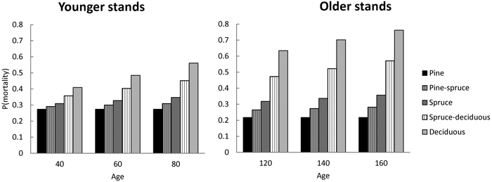
Fig. 1. The predicted probability of mortality during next 5-year period with respect to stand age for stands having different species composition (pure vs 50% mixture). The stand basal area of 23 m2 ha–1, stem number of 970 ha–1 for younger stands and 700 ha–1 for older stands, DQ of 17.4 cm and 20.4 cm, respectively, are reflecting means for the Swedish modelling data group into stands below or above 100 year of stand age.
3.2 Performance of Model 1
The following results are presented in terms of probability of mortality to enable comparison to the earlier studies (Fridman and Ståhl 2001; Eid and Øyen 2003). Analyzing behavior and reliability of Model 1, predicted and observed mortality rates were compared for the total combined dataset. In general, the model predictions were highly correlated with the observed mortality rates. A slight overestimation in the mortality rates can be seen in the oldest stands, when age was above 180 yrs (Fig. 2A) and when DQ was 35–39 cm (Fig. 2B) but, simultaneously, mortality rates were unbiased against DG (Fig. 2C). Predicted mortality rates were also unbiased with respect to stem number (Fig. 3A) and basal area (Fig. 3B). Compared to spruce, larger proportions of pine decreased (Fig. 4B), whereas broadleaved species increased (Fig. 4C) the probability of mortality. Unbiased predictions were also observed for different species mixtures (Fig. 4).
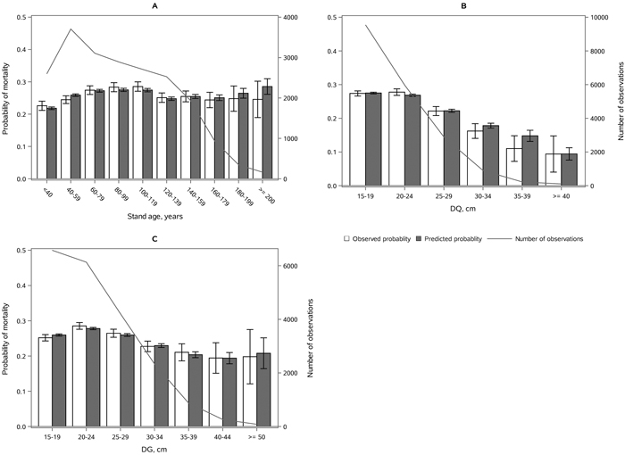
Fig. 2. Observed vs predicted 5-yr probability of mortality (with 95% confidence limits) by classes of A) stand age, B) quadratic mean dbh, DQ and C) basal area weighted mean dbh, DG. The line depicts the number of observations in each class. View larger in new window/tab.
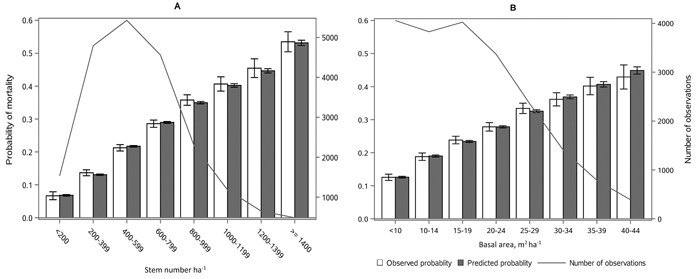
Fig. 3. Observed vs predicted 5-yr probability of mortality (with 95% confidence limits) by classes of A) stem number and B) basal area. The line depicts the number of observations in each class. View larger in new window/tab.
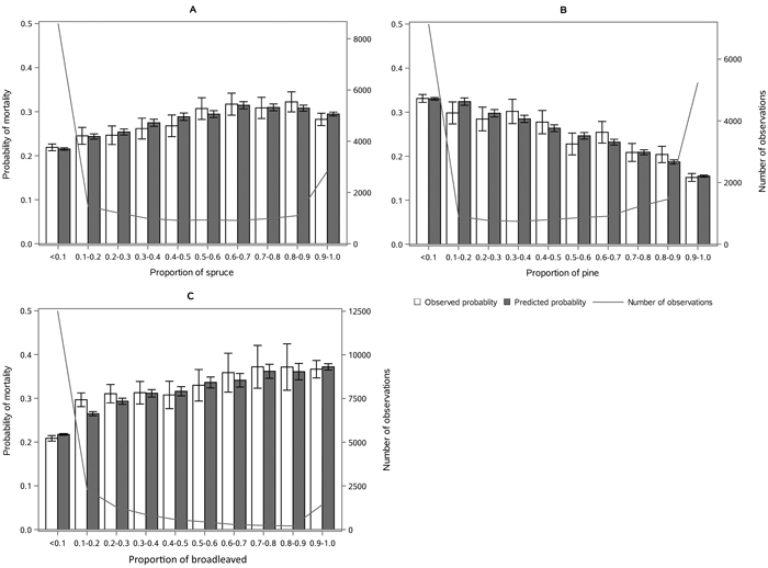
Fig. 4. Observed vs predicted 5-yr probability of mortality (with 95% confidence limits) by classes of A) proportion of spruce, B) proportion of pine and C) proportion of broadleaved species of basal area. The line depicts the number of observations in each class. View larger in new window/tab.
3.3 Basal area of surviving trees (Model 2)
The estimated parameters for Model 2 are presented in Table 6. The weighted RMSE of Model 2 was 0.071 while the mean of response variable P (proportion of basal area in surviving trees) was 0.93. Similar to Model 1, the explanatory variables characterized stand developmental stage (age and DQ), density (N and BA), and species composition. However, many of the explanatory variables had different transformations as compared to Model 1. All the parameter estimates were significant according to 95% confidence limits (Table 6). In this model, site characteristics (peat, moist, dry) or thinnings were not significant. Slope and aspect were significant predictors, but they could not adequately describe the differences between Norway and Sweden. Finally, a categorical variable for west facing slopes and a categorical variable for Norway were used in order to provide unbiased predictions for both countries. They both indicated higher proportion of basal area in survived trees.
| Table 6. Estimated parameters for the linear part (X'b) for the proportion of basal area in surviving trees (Model 2). | ||||
| Variable | Estimate | Approx | Approximate 95% Confidence | |
| Std Error | Limits | |||
| Intercept | –7.3745 | 0.7404 | –8.8259 | –5.9230 |
| ln(N) | 1.4010 | 0.1356 | 1.1351 | 1.6668 |
| √N | –0.0296 | 0.0131 | –0.0554 | –0.0039 |
| BA | –0.0117 | 0.0037 | –0.0190 | –0.0044 |
| ln(DQ) | 0.5633 | 0.1569 | 0.2556 | 0.8709 |
| BApineRel × ln(Age) | 0.0790 | 0.0100 | 0.0595 | 0.0986 |
| BAbrdRel × ln(Age) | –0.0500 | 0.0105 | –0.0706 | –0.0293 |
| Slope/100 × West | 0.2438 | 0.1212 | 0.0062 | 0.4814 |
| NORWAY | 0.1657 | 0.0304 | 0.1060 | 0.2254 |
| NORWAY: dummy variable for Norwegian NFI data. | ||||
In general, the estimated parameters were not highly correlated with each other. However, two high correlations were found 1) between the transformation in stem number, namely ln(N) and square root of N (r = –0.915) and 2) between basal area and quadratic mean diameter (r = –0.879). Nevertheless, the clear non-linear trend in the amount of mortality over stem number required both transformations. The higher the stem number was, the smaller the proportion of basal area of dead trees. This was simply because high density was related to a higher proportion of smaller trees, which were more likely to die because of tree competition. When the mortality was directed to smallest trees the basal area of dead trees was very small. Because of the differences in dynamics between tree species (e.g. growth and senescence), an interaction parameter between stand age and species proportion was significant in this model, too. The estimated parameters showed a pronounced age effect for broadleaved species and a smaller age effect for pine when compared with the model expectation for spruce.
3.4 Performance of Model 2
The following results are presented as an amount of mortality (proportion and absolute basal area of dead trees) to enable comparison to the earlier studies (Fridman and Ståhl 2001; Eid and Øyen 2003). Model 2 showed satisfying behavior against stand developmental stage (Fig. 5), stand density (Fig. 6), and species proportions (Fig. 7). The predicted basal area of dead trees with respect to BA, N and DQ were precise, even though the observed relationships were curvilinear. In the cases, where numbers of observations by groups were low, standard deviations were high. The basal area of dead trees with respect to species proportion was reasonable but there was random variation that was not detected through continuous species proportion, resulting in overestimation in dead basal area when the proportion of pine or broadleaved species was around 15% and 35%. On the other hand, when we classified different species proportions and used them as dummy variables, the model behavior became peculiar with sudden decrease or increase in mortality when stepping from one proportion class to another. In general, when observed and predicted mortality differed considerably in some classes, also the confidence limits were wide, and differences were not significance (see Figs. 5–7).
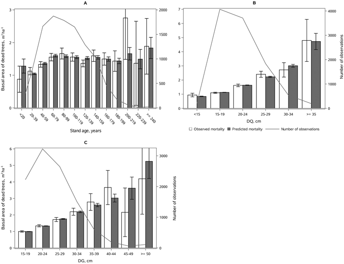
Fig. 5. Mean observed vs mean predicted 5-yr amount of mortality in m2 ha–1 (with 95% confidence limits) by classes of A) age, B) DQ, and C) DG. The line depicts the number of observations in each class. View larger in new window/tab.
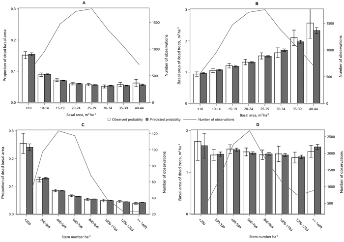
Fig. 6. Mean observed vs mean predicted 5-yr amount of mortality (with 95% confidence limits) as proportion of basal area (Figs. A, C) and absolute basal area of dead trees (Figs. B, D) by classes of stand basal area (Figs. A, B) and stem number (Figs. C, D). The line depicts the number of observations in each class. View larger in new window/tab.
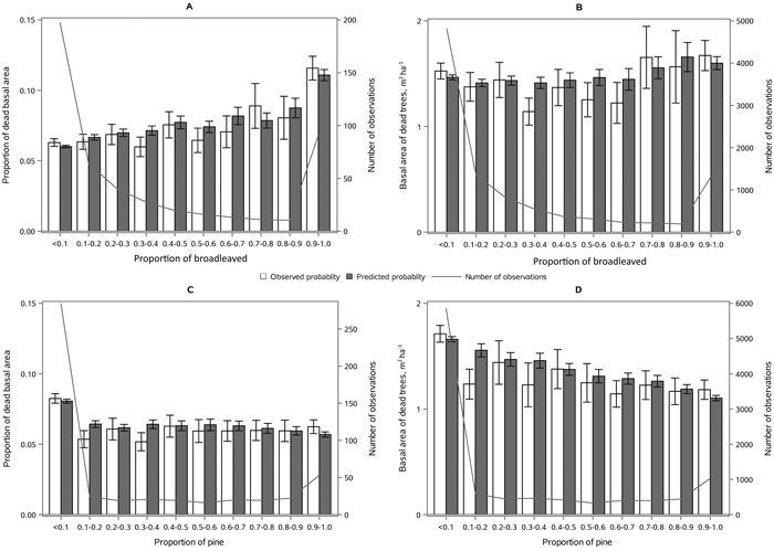
Fig. 7. Mean observed vs mean predicted 5-yr amount of mortality (with 95% confidence limits) as proportion of basal area (A, C) and absolute basal area (B, D) by the proportion of broadleaves (A, B) and proportion of Scots pine (C, D) of stand basal area. The line depicts the number of observations in each class. View larger in new window/tab.
3.5 Application to independent data set
The mean bias in the predicted basal area of dead trees for 57 natural spruce-dominated stands was only –0.051 m2 ha–1 and not significant (Table 7). However, because mortality has a highly stochastic feature, the prediction errors may be large at stand level. As an example, one observation was only 3.0 m2 ha–1 mortality in 11 yrs in the densest stand having BA of 65 m2 ha–1. In this case the prediction of 8.1 m2 ha–1 mortality was an obvious overestimation. On the other hand, for an almost similar plot (BA = 64 m2 ha–1), which had 8.8 m2 ha–1 mortality in 12 yrs, the prediction of 8.6 m2 ha–1 was very close to observed mortality. However, some trends in the prediction errors were found. E.g. the bias with respect to predicted basal area of dead trees (Fig. 8A) showed that the small predictions were mainly underestimations while the greatest predictions were mainly overestimations. Nevertheless, the bias within classes remained always within ± one standard deviation of the prediction error. Other similar trends (not shown here) were found with respect to total basal area and total stem number while opposite trends were found with respect to plot size and mean diameter, DQ and DG. Finally, there was no trend in the residual errors with respect to stand age varying from 80 to 290 yrs (Fig. 8B).
| Table 7. The observed and predicted basal area (BA) of dead trees in the Finnish natural spruce-dominated stands within the observed period length (7–15 yrs) simulated in 5-year steps and the remaining shorter step (e.g. 2-year step when period length was 7 yrs) in Motti. | ||||
| Mean | St. deviation | Minimum | Maximum | |
| Observed BA of dead trees, m2 ha–1 | 3.68 | 2.23 | 0.05 | 10.39 |
| Predicted BA of dead trees, m2 ha–1 | 3.73 | 1.74 | 0.94 | 8.57 |
| Prediction error in the BA of dead trees, m2 ha–1 | –0.051 | 2.48 | –5.25 | 5.68 |
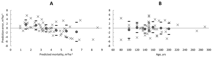
Fig. 8. Prediction errors (× = observed – predicted) in amount of mortality by classes of predicted basal area of dead trees (A) and by classes of stand age (B) in unmanaged spruce dominated stands in Finland. Filled circles showed the average bias within 1-m2 ha–1 basal area and 20-year age classes and thick line showed the ± standard deviation of the prediction error. View larger in new window/tab.
4 Discussion
This study emanated from the need of reliable forecasts of forests with varying structures and varying management regimes. Specifically, it addressed the question of mortality among trees in stands of varying age and with varying degree of within-stand competition. The focus was on predicting mortality of stands, which have already passed the juvenile stage, and in which competition can be described with commonly measured tree and stand characteristics available in forest inventory data. Special emphasis was given to mortality prediction of stand beyond the commercial rotation age.
The plot sizes were rather small in NFI data sets for modelling mortality, which was a disadvantage. However, the clear advantage was the representativeness as well as the large number of plots in the combined NFI data sets. Due to these advantages, we believe that our models could recognize also the possibility of low levels of mortality (Allison 2012). When mortality occurred, the correction factor was calculated for individual tree mortality in order to meet predicted amount of mortality (Fridman and Ståhl 2001). Differences in plot sizes influence the probability and the amount of mortality. Enlarging plot size means increased probability of mortality occurrence but simultaneously, trees represent lower proportion per hectare and thus, a lower amount of mortality. Fridman and Ståhl (2001) were able to estimate the effect of plot size because of high variation in it (78–314 m2). Eid and Øyen (2003) discussed the effect of plot size on probability of mortality but they did not use it as weighting factor. Weighting was applied to account for plot size differences in Sweden and Norway (the relative power). Presumably, this was the first time weighting due to different plot sizes was applied in a logistic function. If the plot size would have been included as explaining variable as in Fridman and Ståhl (2001), the estimated parameter could describe the differences between two countries instead of effect of plot size on the dependent variable. Nevertheless, because the models were fitted to relatively small plots, a relatively large proportion of the trees was affected by the forest condition outside the plot (Eid and Øyen 2003). This means that the estimate for competition become insensitive (underestimate) if we only could compare it with the larger plots as Hynynen and Ojansuu (2003). In practice this means that the mortality will be underestimated if we apply these models to notably larger stand plots than we had in the modelling data (i.e. plot size as a weighting factor could not compensate the fact that estimated parameters of the models would have changed if larger plots were available). Note that Fridman and Ståhl (2001) did not recommend applying their models beyond the plot size used in modelling. Eid and Øyen (2003) stated that their model provided reasonable stand level mortality even ignoring the effect of plot size. Because the plot size had opposite effect on Model 1 and Model 2, ignoring it when predicting the average stand level mortality (deterministic use of the models) may be the best option here as well. Anyhow, even if mortality is the main interest, modelling survival is recommended in order to be able to use a correct weighting for period length and plot size when fitting the model.
When stand-level mortality has been modelled, the typical approach includes two-steps. Woollons (1998) suggested this method to overcome problems due to high number of plots without any mortality. Similarly as in our study, the first step predicts the probability of mortality and the second step predicts the amount of mortality. Even if the reduction in the initial stem number has been more common approach for the amount of mortality (Woollons 1998; Eid and Øyen 2003; Álvarez et al. 2004) than reduction in the initial basal area (Fridman and Ståhl 2001), the latter was preferred. One of the most important structural characteristics for forest biodiversity is the amount and quality of deadwood. It is obvious that basal area of dead wood correlates more closely with the volume of dead wood than the number of dead stems.
If the validation figures are compared with respect to basal area and stem number between Fridman and Ståhl (2001) to presented Model 1, a clear difference can be seen. Combining Norwegian NFI to Swedish NFI in addition to current Swedish NFI measurements resulted in more linear dependence between probability of mortality and stand density. In the models by Fridman and Ståhl (2001) the Swedish NFI data consisted of one or two growth periods, while here the Swedish NFI consisted of four growth periods at best.
The final model structures showed that many of the relationships between response and predictor variables were nonlinear and needed suitable transformation or even combinations of variable transformation. An example was DQ in Model 1 which was finally included as DQ1.5. Using DQ2 resulted in the same AIC, but the behavior with pine and spruce in a simulator was not reasonable. Including DQ with a power was necessary to avoid bias in stand basal area. Another example was the number of stems in Model 2 which was included as natural logarithm of N and square root of N. With these two variables the nonlinearity shown in Fig. 5 was nicely detected.
The differences in mortality between Sweden and Norway were not fully detected with the available stand-level variables in Model 1. There were two variables in the model which could account for some variability between Sweden and Norway, namely slope (5% vs 29%) and occurrence of thinning within 5 years (17% vs 4%). Generally, the model slightly overestimated (0.7%) the probability of mortality occurrence in Sweden and slightly underestimated (1.2%) that in Norway. Nevertheless, we cannot exclude the possibility that in Sweden, dead or dying trees have been removed by land owners more often than in Norway and thus, leading to the underestimation in Sweden. Also the effect of thinning was more minor than expected. Recent thinnings may have two-sided effect, on the one hand thinning decrease the competition between trees which means decreasing probability of mortality but on the other hand, before adapting new conditions trees are exposed to wind and snow damages.
All the broadleaved species were included in one broadleaves group in our NFI data sets. Fridman and Ståhl (2001) divided broadleaved species into three groups, namely birch, other broadleaves (mainly aspen and alder) and southern deciduous (mainly European oak (Quercus robur L.) and European beech (Fagus sylvatica L.)) for tree-level modelling. It is possible that dividing deciduous species into groups could also improve the stand-level models. This is because of the species senescence and thus, mortality rates differed between these broadleaved species groups (Laarmann et al. 2009).
There were considerable differences in site properties and stand structures between Norway and Sweden. E.g. the variation in altitude, temperature sum, slope, stand age and basal area were much higher in Norway. According to model validation, these differences did not show any marked bias in the validation figures for Model I. However, the growing conditions and forest management in Sweden and Finland are quite equal and thus, presented models should be able to predict reasonable mortality rate in Finland.
In order to analyze model behavior in stands without management practices commonly applied in commercial forests, the model performance in dataset including stands which have grown without management for a long period of time was tested. A dataset from Finland consisting of unmanaged spruce stands was used as an independent validation data set (see Peltoniemi and Mäkipää 2011). The analysis revealed an average bias was –0.05 m2 ha–1 which account for 1.4% overestimation. There was no trend in prediction error with respect to stand age (80–300 yrs).
In conclusion, the work was performed as a Nordic co-operation. Stand-level mortality models are now in a stage of implementation into the simulation systems of each country. According to small independent validation data set the presented models provided logical mortality predictions for unmanaged stands, which are notably older than commercial forests on the average.
Acknowledgements
This study was funded by Nordic Forest Research (SNS) project “SNS-122_ Improving Simulation tools for assessing the long-term responses of forest carbon storage to forest management alternatives in Nordic countries”. Additional funding was received also from Natural Resources Institute Finland (Luke), Swedish University of Agricultural Sciences (SLU) and Norwegian Institute of Bioeconomy Research (NIBIO). We thank the anonymous reviewers for helping us to improve the manuscript.
References
Affleck D.L.R. (2006). Poisson mixture models for regression analysis of stand-level mortality. Canadian Journal of Forest Research 36(11): 2994–3006. https://doi.org/10.1139/x06-189.
Allison P. (2012). Logistic regression for rare events. https://statisticalhorizons.com/logistic-regression-for-rare-events. [Cited 6 Oct 2020]
Álvarez J.G., Castedo F., Ruiz A.D., López C.A., Gadow,K.v. (2004). A two-step mortality model for even-aged stands of Pinus radiata D. Don in Galicia (Northwestern Spain). Annals of Forest Science 61(5): 439–448. https://doi.org/10.1051/forest:2004037.
Antón-Fernández C., von Lüpke N., Astrup R. (2019). SiTree: a framework for individual tree simulation. [Manuscript].
Bircher N., Cailleret M., Bugmann H. (2015). The agony of choice: different empirical mortality models lead to sharply different future forest dynamic. Ecological Applications 25(5): 1303–1318. https://doi.org/10.1890/14-1462.1.
Buongiorno J., Gilless J.K. (2003). Decision methods for forest resource management. Academic Press. San Diego, CA, USA. 439 p.
Eid T., Hobbelstad K. (2000). AVVIRK-2000: a large-scale forestry scenario model for long-term investment, income and harvest analysis. Scandinavian Journal of Forest Research 15(4): 472– 482. https://doi.org/10.1080/028275800750172736.
Eid T., Øyen B.-H. (2003). Models for prediction of mortality in even-aged forest. Scandinavian Journal of Forest Research 18(1): 64–77. https://doi.org/10.1080/02827581.2003.10383139.
Eid T., Tuhus E. (2001). Models for individual tree mortality in Norway. Forest Ecology and Management 154(1–2): 69–84. https://doi.org/10.1016/S0378-1127(00)00634-4.
Fahlvik N., Elfving B., Wikström P. (2014). Evaluation of growth models used in the Swedish forest planning system Heureka. Silva Fennica 48(2) article 1013. https://doi.org/10.14214/sf.1013.
Fortin M., Bédard S., DeBlois J., Meunier S. (2008). Predicting individual tree mortality in northern hardwood stands under uneven-aged management in southern Québec, Canada. Annals of Forest Science 65 article 205. https://doi.org/10.1051/forest:2007088.
Fridman J., Ståhl G. (2001). A three-step approach for modelling tree mortality in Swedish forests. Scandinavian Journal of Forest Research 16(5): 455–466. https://doi.org/10.1080/02827580152632856.
Fridman J., Holm; S., Nilsson M., Nilsson P., Ringvall A.H., Ståhl G. (2014). Adapting National Forest Inventories to changing requirements – the case of the Swedish National Forest Inventory at the turn of the 20th century. Silva Fennica 48(3) article 1095. https://doi.org/10.14214/sf.1095.
Hamilton D.A. (1986). A logistic model for mortality in thinned and unthinned mixed conifer stands of northern Idaho. Forest Science 32: 989–1000.
Hanlon B., Larget B. (2011). Statistical analysis of proportions. Department of Statistics. University of Wisconsin–Madison. http://pages.stat.wisc.edu/~st571-1/04-proportions-2.pdf. [Cited 6 Oct 2020].
Hoen H.F., Eid T. (1990). [A model for analysis of treatment strategies for a forest applying standwise simulations and linear programming]. Rapport fra Norsk Institutt for Skogforskning 9/90: 1–35. [in Norwegian with English summary].
Hosmer D.W., Lemeshow S. (1989). Applied logistic regression. John Wiley and Sons, New York. ISBN 0-471-61553-6. 307 p.
Hynynen J., Ojansuu R. (2003). Impact of plot size on individual-tree competition measures for growth and yield simulators. Canadian Journal of Forest Research 33(3): 455–465. https://doi.org/10.1139/x02-173.
Hynynen J., Ojansuu R., Hökkä H., Siipilehto J., Salminen H., Haapala P. (2002). Models for predicting stand development in MELA system. Finnish Forest Institute, Research Papers 835, Vantaan Research Center. 116 p. http://urn.fi/URN:ISBN:951-40-1815-X.
Isomäki A., Niemistö P., Varmola M. (1998). Luonnontilaisten metsien rakenne seurantakoealoilla. [Structure of the natural forests on monitoring plots]. Metsäntutkimuslaitoksen Tiedonantoja 705: 75–86. http://urn.fi/URN:ISBN:951-40-1647-5.
Jutras S., Hökkä H., Alenius V., Salminen H. (2003). Modeling mortality of individual trees in drained peatland sites in Finland. Silva Fennica 37(2): 235–251. https://doi.org/10.14214/sf.504.
Kaipainen T., Liski J., Pussinen A., Karjalainen T. (2004). Managing carbon sinks by changing rotation length in European forests. Environmental Science & Policy 7(3): 205–219. https://doi.org/10.1016/j.envsci.2004.03.001.
Keenan R.J. (2015). Climate change impacts and adaptation in forest management: a review. Annals of Forest Science 72: 145–167. https://doi.org/10.1007/s13595-014-0446-5.
Laarmann D., Korjus H., Sims A., Stanturf J.A., Kiviste A., Körster K. (2009). Analysis of naturalness and tree mortality patterns in Estonia. Forest Ecology and Management 258: S187−S195. https://doi.org/10.1016/j.foreco.2009.07.014.
Lämås T., Eriksson L.O. (2003). Analysis and planning systems for multiresource, sustainableforestry: the Heureka research programme at SLU. Canadian Journal of Forest Research 33(3): 500–508. https://doi.org/10.1139/x02-213.
Lee Y. (1971). Predicting mortality for even-aged stands of lodgepole pine. Forestry Chronicle 47(1): 29–32. https://doi.org/10.5558/tfc47029-1.
Lundmark T., Bergh J., Nordin A., Fahlvik N., Poudel B.C. (2016). Comparison of carbon balance between continuous-cover and clear-cut forestry in Sweden. Ambio 45: 203–213. https://doi.org/10.1007/s13280-015-0756-3.
McCulloch C.E., Searle S.R., Neuhaus J.M. (2008). Generalized, linear, and mixed models. 2nd ed. Wiley Series in Probability and Statistics. John Wiley and Sons, Hoboken, New York.
Mehtätalo L., Lappi J. (2020). Biometry for forestry and environmental data with examples in R. Chapman & Hall/CRC. Applied Environmental Series. https://doi.org/10.1201/9780429173462.
Monserud R. (1976). Simulation of forest tree mortality. Forest Science 22: 438–444.
Monserud R., Sterba H. (1999). Modelling individual tree mortality for Austrian forest species. Forest Ecology and Management 113(2–3): 109–123. https://doi.org/10.1016/S0378-1127(98)00419-8.
Peltoniemi M., Mäkipää R. (2010). Quantifying distance-independent tree competition for predicting Norway spruce mortality in unmanaged forests. Forest Ecology and Management 261(1): 30–42. https://doi.org/10.1016/j.foreco.2010.09.019.
Salas-Eljatib C., Weiskittel A.R. (2020). On studying the patterns of individual-based tree mortality in natural forests: A modelling analysis. Forest Ecology and Management 475 article 118369. https://doi.org/10.1016/j.foreco.2020.118369.
SAS 9.4 Product documentation. https://support.sas.com/documentation/94/. [Cited 2 Dec 2019].
Siitonen M. (1995). The MELA system as a forestry modelling framework. Lesnitcy-Forestry 41: 173–178.
Siitonen M., Nuutinen T. (1996). Timber production analyses in Finland and MELA system. In Päivinen R., Roihuvuo L., Siitonen M. (eds.). Large-scale forestry scenario models: experiences and requirements. Proceedings of the international seminar and summer school, 15–22 June 1995, Joensuu, Finland. EFI Proceedings No. 5. p. 89–98.
Sims A., Mändma R., Laarman D., Korjus H. (2014). Assessment of tree mortality on Estonian Network of Forest Research Plots. Forestry Studies | Metsanduslikud Uurimused 60(1): 57–68. https://doi.org/10.2478/fsmu-2014-0005.
Söderberg, Ulf (1992). Funktioner för skogsindelning: höjd, formhöjd och barktjocklek för enskilda träd. [Functions for forest management : height, form height and bark thickness of individual trees]. Sveriges lantbruksuniversitet, Umeå.
Taylor A.R., Chen H.Y.H., VanDamme L. (2009). A review of forest succession models and their suitability of forest management planning. Forest Science 55(1): 23–36.
Tomter S., Hylen G., Nilsen J. (2010). National forest inventory report: Norway. In: Tomppo E., Gschwantner T., Lawrence M., McRoberts R.E. (eds.). National forest inventories. Pathways for common reporting. Springer, Heidelberg. p. 411–424.
Tuominen S., Pitkänen J., Balazs A., Korhonen K.T., Hyvönen P., Muinonen E. (2014). NFI plots as complementary reference data in forest inventory based on airborne laser scanning and aerial photography in Finland. Silva Fennica 48(2) article https://doi.org/10.14214/sf.983.
Vanclay J. (1991). Mortality functions for north Queensland rainforests. Journal of Tropical Forest Science 4(1): 15–36. https://www.jstor.org/stable/43594423.
Vanclay J. (1994). Modelling forest growth and yield. Applications to mixed and tropical forests. CAB International. 312 p.
Verkaik E., Nabuurs G.J. (2000). Wood production potentials of Fenno-Scandinavian forests under nature-orientated management. Scandinavian Journal of Forest Research 15(4): 445–454. https://doi.org/10.1080/028275800750172673.
Vieilledent G., Courbaud, Kunstler G. Dhote J.F., Clark J.S. (2009). Biases in the estimation of size-dependent mortality models: advantages of a semiparametric approach. Canadian Journal of Forest Research 39(8): 1430–1443. https://doi.org/10.1139/X09-047.
Weiskittel A.R., Hann D.W., Kershaw J.A., Vanclay J.K. (2011). Forest growth and yield modeling. John Wiley & Sons. 451 p. https://doi.org/10.1002/9781119998518.
Woollons R.C. (1998). Even-aged stand mortality through a two-step regression process. Forest Ecology and Management 105(1–3): 189–195. https://doi.org/10.1016/S0378-1127(97)00279-X.
Yli-Kojola H. (2005). Metsikkö- ja puutuhojen ennustemallit. [Prediction models for stand- and tree-level damages]. Metsäntutkimuslaitoksen tiedonantoja 948. 122 p. http://urn.fi/URN:ISBN:951-40-1989-X.
Total of 48 references.
