Daniel Schraik  ,
Aarne Hovi,
Miina Rautiainen
,
Aarne Hovi,
Miina Rautiainen
Estimating cover fraction from TLS return intensity in coniferous and broadleaved tree shoots
Schraik D., Hovi A., Rautiainen M. (2021). Estimating cover fraction from TLS return intensity in coniferous and broadleaved tree shoots. Silva Fennica vol. 55 no. 4 article id 10533. https://doi.org/10.14214/sf.10533
Highlights
- We developed a method to obtain the fraction of TLS pulses’ footprint area covered by a target’s projection area
- We tested our method with shoots of Norway spruce, Scots pine and silver birch
- We provide a physically-based framework related to unmeasured variables, and provide a robust statistical framework to deal with uncertainty.
Abstract
Terrestrial laser scanning (TLS) provides a unique opportunity to study forest canopy structure and its spatial patterns such as foliage quantity and dispersal. Using TLS point clouds for estimating leaf area density with voxel-based methods is biased by the physical dimensions of laser beams, which violates the common assumption of beams being infinitely thin. Real laser beams have a footprint size larger than several millimeters. This leads to difficulties in estimating leaf area density from light detection and ranging (LiDAR) in vegetation, where the target objects can be of similar or even smaller size than the beam footprint. To compensate for this bias, we propose a method to estimate the per-pulse cover fraction, defined as the fraction of laser beams’ footprint area that is covered by vegetation targets, using the LiDAR return intensity and an experimental calibration measurement. We applied this method to a Leica P40 single-return instrument, and report our experimental results. We found that conifer foliage had a lower average per-pulse cover fraction than broadleaved foliage, indicating an increased number of partial hits in conifer foliage. We further discuss limitations of our method that stem from unknown target properties that influence the LiDAR return intensity and highlight potential ways to overcome the limitations and manage the remaining uncertainty. Our method’s output, the per-beam cover fraction, may be useful in a weight function for methods that estimate leaf area density from LiDAR point clouds.
Keywords
terrestrial laser scanning;
leaf area;
lidar intensity;
physically-based;
voxel
-
Schraik,
Aalto University, School of Engineering, Department of Built Environment, P.O. Box 14100, FI-00076 Aalto, Finland;
 https://orcid.org/0000-0002-7794-3918
E-mail
daniel.schraik@aalto.fi
https://orcid.org/0000-0002-7794-3918
E-mail
daniel.schraik@aalto.fi
-
Hovi,
Aalto University, School of Engineering, Department of Built Environment, P.O. Box 14100, FI-00076 Aalto, Finland;
https://orcid.org/0000-0002-4384-5279
E-mail
aarne.hovi@aalto.fi
-
Rautiainen,
Aalto University, School of Engineering, Department of Built Environment, P.O. Box 14100, FI-00076 Aalto, Finland; Aalto University, School of Electrical Engineering, Department of Electronics and Nanoengineering, P.O. Box 14100, FI-00076 Aalto, Finland
https://orcid.org/0000-0002-6568-3258
E-mail
miina.a.rautiainen@aalto.fi
Received 3 March 2021 Accepted 24 August 2021 Published 30 August 2021
Views 22052
Available at https://doi.org/10.14214/sf.10533 | Download PDF

Supplementary Files
1 Introduction
Terrestrial laser scanning (TLS) is increasingly used in estimating leaf area of forest stands, for which it is uniquely suited due to its ability to create highly detailed three-dimensional representations of forest trees and stands. The level of detail in TLS measurements paved the way for studies of forest canopy structure that previously could be done only with costly destructive methods or were impossible altogether.
A promising approach to derive forest canopy structural properties from point clouds is based on estimating the leaf area density on a voxel grid by means of ray tracing (e.g., Béland et al. 2014; Pimont et al. 2018). Viewing a pulse in a TLS point cloud as a ray which ends at the point of hitting a target, one can calculate the leaf area density based on the number of intercepted and transmitted rays in a voxel. This method of estimating leaf area density has been applied to real trees and branches (Soma et al. 2018; Schraik et al. 2021), which indicated estimation biases in practice.
An important challenge to TLS-based leaf area estimation using the above described voxel-based approach is the beam size effect. The approach assumes that the laser beam has an infinitesimal size. In practice, in a typical TLS measurement, beam size ranges from the order of millimeters up to several centimeters. This can be problematic since vegetation elements that are not centered on a beam may trigger a return. These partial hits violate the assumption of infinitesimal beam size and may cause overestimation in leaf area density. We investigated a way to account for such partial hits from a physical perspective and propose a method to correct light detection and ranging (LiDAR) data to yield the fraction of the beam footprint that is covered by vegetation elements using only the return intensity and species information.
According to the LiDAR equation (Wagner et al. 2006), the return intensity depends on target and instrument characteristics, atmospheric attenuation, and scan range. Assuming that the emitted pulse power is constant, and the receiver’s response is linear, and ignoring the atmosphere, the range-corrected intensity (i.e., intensity normalized to some arbitrary reference range Rref by multiplying with R2/Rref2) is a linear measure of the target’s backscattering coefficient (Wagner 2010). The backscattering coefficient depends on the target’s reflectance, directional scattering characteristics, and cover fraction, i.e., the area fraction of the LiDAR footprint that hits a target. At constant reflectance and directional scattering characteristics, intensity depends only on cover fraction, and therefore the cover fraction can be predicted based on the measured intensity. Because the cover fraction is only defined between zero and one, the use of linear regression is invalid, and beta regression may be used instead (Ferrari and Cribari-Neto 2004). However, a solution to the cover fraction can be achieved only up to uncertainty of the unknown parameters, i.e. the reflectance and directional scattering characteristics.
In this study, we propose a method to estimate the cover fraction (defined here as TLS footprint area that is covered by vegetation targets) based solely on the return intensity. We applied this method to measurements of individual shoots of trees with a single-return TLS instrument and quantified the intensity-cover fraction relationship for different tree species, while explicitly accounting for uncertainty originating from unknown target properties. Our method is intended to provide a correction term for leaf area density estimation methods by relaxing the assumption of infinitesimal beam diameter, and instead using the per-pulse cover fraction to quantify the number of vegetation hits inside a voxel.
2 Materials and methods
2.1 Measurements
We built a simple wooden construction that held six shoots suspended, i.e. with lines of sight not intersecting both the shoots and the frame (Fig. 1). The shoots were attached to the frame with cotton thread. Five Leica 4.5” B&W registration targets were attached on the frame around the shoots. The construction was attached to a tripod, and it could be rotated up to 45 degrees off perpendicular without the frame occluding the shoots. We sampled 18 shoots of each of the common Finnish tree species Scots pine (Pinus sylvestris L.), Norway spruce (Picea abies (L.) H. Karst.) and silver birch (Betula pendula Roth). The samples were taken from stand edges in Espoo (Finland), from up to 2 m above ground. The site type for pine was sub-xeric, and for spruce and birch mesic.
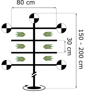
Fig. 1. Schematic of the shoot holder that was used to suspend shoots in the experiment. The shoots were fixed to the frame with thread.
The measurements consisted of TLS scans (Leica P40) at 0.8 mrad scan resolution (0.8 mm at 10 m distance) and reference photographs using a Sony A7R camera and an 80–200 mm f4 lens, taken from the same position with a tolerance of 5 cm. Measurements were taken at distances of 5, 10, 15 and 20 m. To capture angular variation, the measurements were made from perpendicular-to-shoot-axis direction, and 45° towards the left and right, respectively. We processed the TLS point clouds into both range and intensity images, that is, arranging the individual LiDAR returns by their polar coordinates to form an image from the scanner’s perspective, with image resolution corresponding to the angular scan resolution, and pixel values corresponding to scan range and intensity, respectively.
We used a radiometric reference target (Spectralon panel with 99% nominal reflectance) in all scans to evaluate range-dependence of the intensity. The intensity was already range-corrected by the instrument, i.e., it was constant with respect to range, with a mean of 0.861 and standard deviation of 0.013. We also investigated the offset and linearity of the intensity scale by performing a scan of gray-level targets (nominal reflectance values of 2–99%), which showed that the scanner’s response was near linear for the intensity range we observed in data from the shoots (I < 0.5), but with increasing nonlinearity upwards from 60% reflectance.
2.2 Methods
The method we propose for estimating the tree species-specific relationship between LiDAR intensity and cover fraction is to (1) identify registration targets in both the intensity/range image and a reference photograph, (2) estimate a projective transformation, and (3) select photo pixels within an approximated area of the beam footprint (Fig. 2). The Python code for this method is in Supplementary file S1.
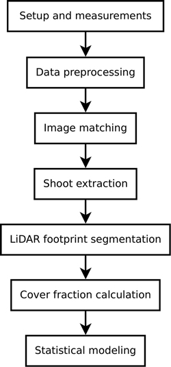
Fig. 2. Flowchart of the proposed method. After measurements and data preprocessing is complete, the TLS intensity image and reference photographs are matched using five targets. Shoot pixels are extracted from the intensity image, and subsequently each LiDAR return’s footprint that comes from a shoot is segmented in the reference photograph. The segmented photograph is then used to calculate the per-pulse cover fraction, and the data is used to create a regression model to predict cover fraction from TLS return intensity.
We manually selected the registration targets from the intensity image and the reference photograph on sub-pixel level. A projective transformation (affine + perspective transform) was used to convert photo coordinates to intensity image coordinates, with residuals less than 3 pixels in the photograph. Then, we manually selected the shoot pixels from the intensity image and filtered the selection based on the range image to exclude LiDAR returns originating from the background. Pixels closer than approximately 2 cm to the wooden frame were excluded. The shoot pixels in the photographs were thresholded using Otsu’s method as a starting point, and then adapting the threshold value downward, up to a factor of 0.7, until the background around the shoots was excluded. This was necessary due to occasionally heterogeneous illumination of the background. Visual examination of the photographs showed negligible effects of this procedure on the shoot silhouette due to the high contrast to the background, and the high resolution of the photograph.
We defined the TLS beam footprint as a beam of finite size at instrument (3.5 mm according to specifications), which increases in size over distance by the beam divergence (0.23 mrad). At the target, we calculated the beam radius as:
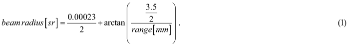
For each TLS return on the shoots, we selected the thresholded photo pixels around the pulse center that were within the beam radius. The per-pulse cover fraction is the mean of thresholded photo pixels where a plant pixel has value 1, and a background pixel has value 0.
The cover fraction is defined between zero and one, therefore we used one-inflated beta regression to quantify the relationship between cover fraction and intensity per species. That is, the cover fraction is modeled as a beta distribution, parameterized with mean and precision (inverse variance). We used a link function to estimate the mean (Ferrari and Cribari-Neto 2004), with the added physical constraint that at zero intensity, the mean cover fraction equals zero. To this end, we modified the commonly used inverse-logit transformation to estimate the mean cover fraction μcf from intensity I as:

with the regression parameter α and an additional parameter for the precision (not shown). Since the beta distribution is bound to the open interval (0,1), inflating the beta regression for unit cover fraction is needed. That is, we estimated an additional parameter, namely the probability that the cover fraction equals one p = Pr(cf = 1), using the standard inverse-logit function p = exp(β0 + β1 I) / (exp(β0 + β1 I) + 1), with the regression parameters β0 and β1. Since zero intensity and cover fraction is physically impossible, as such a case would not trigger a return, we ignored the lower boundary of the beta distribution. To summarize, the mean of the response variable as a function of the predictor was calculated as μcf ‘ = μcf (1 – p) + p.
We used a Bayesian approach to infer the unknown parameters from the data. We chose vague, normally distributed priors N(μ,σ) for all parameters, that are, Pr(α) = N(0,50), Pr(precision) = N(0,50) for precision > 0, and Pr(β0) = Pr(β1) = N(0.5,1). Given the large amount of data, these priors had a negligible effect on the posterior.
We used the Stan implementation of Markov-Chain Monte Carlo (Stan Development Team 2021) to take 2000 samples in each of 4 chains from the joint posterior distribution, using 1% of the available data (39 106 pulses). Then, we sampled from the posterior predictive distribution, i.e., the probability distribution for predicting a new observation, for the remaining 99% of the data (3 862 505 pulses). We summarize the posterior and posterior predictive distributions using means and credible intervals (CI), which we define as the narrowest interval that contains a specified percentage of the parameters probability distribution. The Stan code for our statistical model is in Suppl. file S2.
3 Results
We obtained about 3.9 million observations of LiDAR return intensity and corresponding cover fraction, of which spruce made up 1.08 million, pine 1.42 million, and birch 1.40 million. Intensity values ranged from 0.02 to 0.76, and the means for spruce and pine were 0.14 and 0.15, respectively, while birch had a mean of 0.26. Cover fraction ranged from 0.02 to 1, with means of 0.86, 0.82, and 0.94 for spruce, pine, and birch, respectively (Fig. 3). Intensity values below about 0.1 were heavily thinned by the TLS instrument, due to the single return processing, which favored the background when the shoot was only partially hit below an unknown threshold, as illustrated in Fig. 4. Furthermore, partial hits were more common in the conifer species, where 54% (spruce) or 63% (pine) of the observations had cover fraction less than 0.9, while in birch it was only 21%.
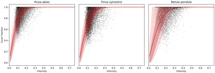
Fig. 3. Scatterplot of cover fraction against TLS return intensity with prediction by beta regression for our study species. The red line indicates the mean of the posterior predictive distribution, and the dark and light red areas indicate the 50% and 90% credible intervals, respectively. The data points were thinned to 1% of the original density. View larger in new window/tab.
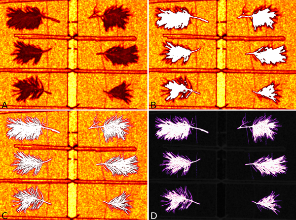
Fig. 4. Illustration of Pinus sylvestris shoots visible by the TLS. A. The intensity image of shoots. B. Points located on the shoot were colored white. C. The shoot silhouette from the thresholded photograph was colored white. D. Difference between the thresholded photograph and the shoot points, with the white area highlighting a match in both images and purple indicating shoot portions only covered by the photograph.
The regression coefficients α for spruce, pine and birch had means of 18.5, 15.8 and 11.0, respectively. All 90% credible intervals were ±0.1 of their mean. The precision parameter was highest for spruce at 7.45 ± 0.15 (CI), and pine at 6.71 ± 0.11, while birch had lower precision at 4.43 ± 0.12. The regression parameters for the one-inflation were β0 = –3.52 ± 0.12 and β1 = 10.88 ± 0.67 for spruce, β0 = –3.95 ± 0.11 and β1 = 12.02 ± 0.60 for pine, and β0 = –2.69 ± 0.08 and β1 = 13.03 ± 0.34 for birch.
The predictions for the data not used in fitting the model had a mean prediction error of –0.01 across all species, that is, the average prediction was slightly lower than the observed values. The root mean square deviation was 0.12 for spruce and birch, and 0.14 for pine. The 90% credible intervals of the predictions contained 83% of the observations for spruce and pine, and 90% of the observations for birch.
4 Discussion
We propose a method to estimate the cover fraction of individual TLS beams based only on the LiDAR return intensity. The intended purpose of this method is to compensate for beam size effects in TLS-based methods to estimate leaf area density. Our method’s estimated cover fraction may be used as a weight function that accounts for partial hits with foliage.
Our method was conceived as an inversion of the LiDAR equation with respect to the fraction of the footprint area covered by a plant target, i.e., the cover fraction. As such, there are obvious limitations with respect to unknown or not readily measurable parameters of the LiDAR equation (optical properties and geometry of vegetation elements) and the instrument (spatial distribution of irradiance within the laser beam). We used Bayesian analysis to explicitly point out the uncertainty inherent to our method. We showed that our statistical analysis resulted in negligible bias. Each cover fraction prediction had considerable uncertainty, indicated by the root mean square deviation of around 0.12. However, we also showed that the 90% credible intervals of the cover fraction predictions included the observed values in a vast majority of cases. This indicates that cover fraction predictions from our method be best interpreted probabilistically, as this preserves the inherent prediction uncertainty due to unknown parameters.
A limitation in our experimental setup was that intensity values in the low range were unobserved. This was caused by single return TLS signal processing, which assigns a return to the background rather than the plant target if the return intensity of the background is larger than the target’s. This led to a lack of observations of intensity values below about 0.1, for which our statistical analysis cannot provide credible predictions. However, our data comprised almost the full range of possible cover fraction values, and the theoretical framework we used should be able to support applicability of our method for lower intensity values. In order to calibrate an instrument with our method, we recommend to use two different background materials, namely a dark background for TLS measurements, and a bright background for photographs. Furthermore, we theorize that this issue is more prominent in conifers than broadleaved tree species due to the former’s larger proportion of partial hits.
While in a real forest partial hits can occur between two vegetation targets, the effect would likely be less pronounced than in our experiment, which required a bright background for the photographs. However, the omission of partial hits around edges should be investigated to quantify its influence on both our method in particular and estimates of leaf area density from TLS data in general.
The method we propose can be applied to any TLS instrument, and we believe that it would prove useful for multi-return and full waveform scanners, which are less susceptible to the partial hit omission mentioned above. The output of our method, the cover fraction, may serve to improve leaf area density estimates by allowing the modeler to apply a weighting function that assigns different weights to full and partial hits. Assigning weights based on cover fraction may help alleviate bias in leaf area density estimation caused by the discrepancy between the assumed infinitesimal and a real TLS footprint size.
Declaration of openness of research materials, data, and code
The data used in this study may be requested from the corresponding author via email. The code is provided in the supplements.
Authors’ contributions
Daniel Schraik conceived the research idea, planned the study, carried out the measurements, data processing and statistical analysis, and wrote the work. Aarne Hovi and Miina Rautiainen refined the research idea into more concrete terms, planned the study, assisted in data processing and statistical analysis, contributed to the report and critically reviewed it.
Acknowledgements
The authors received funding from the European Research Council (ERC) under the European Union’s Horizon 2020 research and innovation programme (grant agreement No 771049). The article reflects only the authors’ view and the Agency is not responsible for any use that may be made of the information it contains.
References
Béland M, Baldocchi DD, Widlowski JL, Fournier RA, Verstraete MM (2014) On seeing the wood from the leaves and the role of voxel size in determining leaf area distribution of forests with terrestrial LiDAR. Agric For Meteorol 184: 82–97. https://doi.org/10.1016/j.agrformet.2013.09.005.
Ferrari S, Cribari-Neto F (2004) Beta regression for modelling rates and proportions. J Appl Stat, 31: 799–815. https://doi.org/10.1080/0266476042000214501.
Pimont F, Allard D, Soma M, Dupuy JL (2018) Estimators and confidence intervals for plant area density at voxel scale with T-LiDAR. Remote Sens Environ 215: 343–370. https://doi.org/10.1016/j.agrformet.2013.09.005.
Schraik D, Hovi A, Rautiainen M (2021) Crown level clumping in Norway spruce from terrestrial laser scanning measurements. Agric For Meteorol 296, article id 108238. https://doi.org/10.1016/j.agrformet.2020.108238.
Soma M, Pimont F, Durrieu S, Dupuy JL (2018) Enhanced measurements of leaf area density with T-LiDAR: evaluating and calibrating the effects of vegetation heterogeneity and scanner properties. Remote Sens 10, article id 1580. https://doi.org/10.3390/rs10101580.
Stan Development Team (2021) Stan, modeling language users guide and reference manual, 2.26. https://mc-stan.org.
Wagner W, Ullrich A, Ducic V, Melzer T, Studnicka N (2006) Gaussian decomposition and calibration of a novel small-footprint full-waveform digitising airborne laser scanner. ISPRS J Photogramm 60: 100–112. https://doi.org/10.1016/j.isprsjprs.2005.12.001.
Total of 7 references.
