Victor F. Strîmbu  ,
Tron Eid,
Terje Gobakken
,
Tron Eid,
Terje Gobakken
A stand level scenario model for the Norwegian forestry – a case study on forest management under climate change
Strîmbu V. F., Eid T., Gobakken T. (2023). A stand level scenario model for the Norwegian forestry – a case study on forest management under climate change. Silva Fennica vol. 57 no. 2 article id 23019. https://doi.org/10.14214/sf.23019
Highlights
- GAYA 2.0: a new scenario analysis model focusing on forest carbon fluxes
- Carbon sequestration potential estimated at regional level
- GAYA 2.0 may be used to estimate the costs of obtaining carbon benefits by adapting the forest management.
Abstract
Carbon sequestration and income generation are competing objectives in modern forest management. The climate commitments of many countries depend on forests as carbon sinks which must be quantified, monitored, and projected into the future. For projections we need tools to model forest development and perform scenario analyses to assess future carbon sequestration potentials under different management regimes, the expected net present value of such regimes, and possible impacts of climate change. We propose a scenario analysis software tool (GAYA 2.0) that can assist in answering these types of questions using stand level simulations, detailed carbon flow models and an optimizer. This paper has two objectives: (1) to describe GAYA 2.0, and (2) demonstrate its potential in a case study where we analyze the forest carbon balance over a region in Norway based on national forest inventory sample plots. The tool was used to map the optimality front between the carbon benefit and net present value. We observed changes in net present value for different levels of carbon benefit as well as changes in optimal management strategies. We predicted future changes in several forest carbon pools as well as albedo and illustrated the impact of gradual increase in forest productivity (i.e., due to climate warming). Having been updated and modernized from its previous version with increased attention to forest carbon and energy fluxes, GAYA 2.0 is an effective tool that offers multiple opportunities to perform various types of scenario analyses in forest management.
Keywords
forest planning;
carbon balance;
climate change mitigation;
forest stand simulator
-
Strîmbu,
Norwegian University of Life Sciences, Faculty of Environmental Sciences and Natural Resource Management, NO-1432 Ås, Norway
 https://orcid.org/0000-0002-0588-2036
E-mail
victor.strimbu@nmbu.no
https://orcid.org/0000-0002-0588-2036
E-mail
victor.strimbu@nmbu.no
- Eid, Norwegian University of Life Sciences, Faculty of Environmental Sciences and Natural Resource Management, NO-1432 Ås, Norway E-mail tron.eid@nmbu.no
-
Gobakken,
Norwegian University of Life Sciences, Faculty of Environmental Sciences and Natural Resource Management, NO-1432 Ås, Norway
https://orcid.org/0000-0001-5534-049X
E-mail
terje.gobakken@nmbu.no
Received 31 March 2023 Accepted 21 August 2023 Published 24 August 2023
Views 71445
Available at https://doi.org/10.14214/sf.23019 | Download PDF

Supplementary Files
1 Introduction
Since the Paris Agreement, global discussions on climate change mitigation have revolved around achieving net zero emissions and limiting warming to 1.5 °C. The Intergovernmental Panel on Climate Change (IPCC) has concluded that the net greenhouse gases emissions should reach zero by around 2050 to limit warming to 1.5 °C. (Pachauri et al. 2014). Many countries, representing over two thirds of the world’s economy, have set net-zero targets (Fankhauser et al. 2022; Hale et al. 2022). However, a recent review shows that despite including forests in their strategies, few countries have quantified their role in reaching net zero emissions (Smith et al. 2022).
Alongside worldwide agreements, national and supranational entities, such as the European Union, implement strategies that are more ambitious, with clearer goals and better leveraged. In 2021, the EU Commission unveiled the New EU Forest Strategy for 2030. This strategy, which blends voluntary actions with regulatory and fiscal measures, is targeted at reducing emissions by 55% by 2030 (EU Comission 2021). Norway mirrored this objective (Government of Norway 2022) and in addition is increasing forest certification requirements from 2023, emphasizing sustainable practices like selective cutting and conservation (PEFC 2022).
The updated climate commitments and new regulations are expected to put more pressure on the forest sector to accommodate climate benefits. There is a call for transformation in forest management, shifting from a predominantly economic focus to include environmental conservation and climate mitigation. Forest management in Europe varies due to unique geographical and socio-economic factors in each country. Therefore, any changes to forest management should be tailored to individual countries or regions. To understand the intricate relationships between forest management and climate scenarios, and to potentially incorporate new government policies and certification regimes, precise and regional simulation tools are needed.
GAYA is a stand-level forest simulator developed for the Norwegian forest sector (Hoen and Eid 1990; Hoen and Gobakken 1997). By itself, it can be used to generate and simulate a set of alternative treatment schedules for each treatment unit (stand or sample plot). Coupled with an optimizer, J (Lappi 2003), it has been a powerful and reliable tool for scenario analyses with detailed insights in the effects of different management regimes. Several studies over the past decades have used GAYA to analyze the relation and effects of competing forest management objectives such as maximizing the net present value and maximizing the carbon sequestration potential (Hoen and Solberg 1994; Hoen and Solberg 1997; Raymer et al. 2009). The simulator has seen several updates and improvements over time but its old FORTRAN code base presents challenges to maintenance and further development. For this reason, there is need for a GAYA version 2.0 with a new, modern, and updated follow-up software. In the new version some of the core models have been improved and updated, including more robust dominant height development models, an updated soil carbon model, and a more detailed carbon accounting module. Furthermore, the wood volume calculations are now based on taper models that improve predictions on the usable stem wood, its monetary value, and the associated carbon flows. GAYA 2.0 has a strong focus on forest carbon fluxes and an added albedo model complementing the range of climate services relevant for boreal forests.
This paper has two main objectives: (1) to describe the new forest stand simulator GAYA 2.0, and (2), to demonstrate the functionality if the software system in a case study that considers the carbon storage potential of the forest on a regional scale. In the case study we aim to quantify the carbon sequestration potential under different silvicultural regimes, estimate costs for different levels of carbon benefits, and illustrate how forest management regimes may change to accommodate increasing levels of carbon benefits. In addition, we show possible effects of gradual increase in boreal forest productivity due to climate warming and predict changes in forest albedo.
2 Software system
GAYA 2.0 was developed using C++ (17 standard), NetBeans IDE (Oracle Corporation 2018), and the MinGW-w64 environment and compilers (Free Software Fundation Inc. 2020). For parallel processing we use the OpenMP API (OpenMP Architecture Review Board 2015). We distinguish two parts of the proposed software system. The main component is the stand simulator which is used to generate alternative treatment schedules for a set of forest stands. Then, connected to this, the optimizer selects the best set of treatments according to an objective function and a set of constraints. GAYA 2.0 uses JLP22 optimizer (Lappi 2022) which is an updated version of the linear programming optimizer J (Lappi 2003). JLP22 was published on GitHub (https://github.com/juhalappi/Jlp22) and is integrated with GAYA 2.0 at the compilation stage. In Fig. 1 we show a concise overview of the system based on a typical use case.
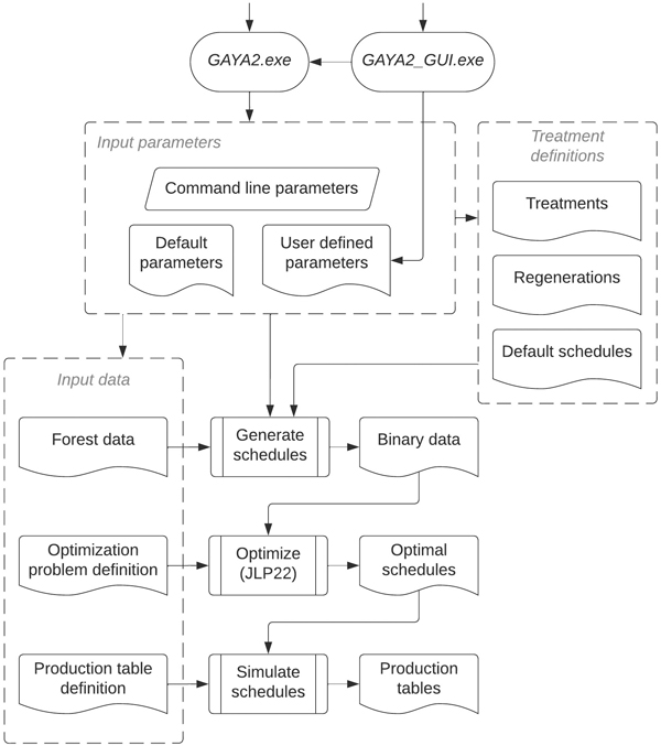
Fig. 1. Software system overview of the GAYA 2.0 forest stand simulator.
GAYA 2.0 may be run directly from the command line or through a simple user interface that facilitates the specification of some basic parameters. The command line option may be used to write batch command files when performing series of simulations with different input data or parameters.
GAYA 2.0 simulations are based on parameters that define forest stand-level attributes. Some of the parameters, represent stand-level means (e.g., mean height, mean diameter, etc.), some are expressed in terms of per hectare (ha–1) values (e.g., number of stems, basal area, volume, etc.), and others are derived from other parts of the stand’s overall distribution of tree metrics (e.g., dominant height). Stands are assumed to host a mix of the three main tree species in Norway: Norway spruce (Picea abies (L.) Karst.), Scots pine (Pinus sylvestris L.), and birch (Betula pendula Roth and Betula pubescens Ehrh.). The biometric values for the species present in a stand are maintained separately. A list of the variables in GAYA 2.0 is given in Supplementary file S1.
Before the simulations, the user provides a set of stand or sample plot data that describe biophysical and logistic attributes, such as the number of stems, dominant height, mean diameter, age, site index, transport distances, and terrain features impacting the cost of harvesting.
Further, the user defines a set of treatments by specifying: (1) conditions based on stand (or sample plot) variables that control when the treatment can be applied, and (2) parameters that define the effect of the treatment on the stand. Each treatment has a conditional statement that must be satisfied before the treatment is allowed as an alternative (e.g., minimum age for harvest), and optionally, a condition that would make the treatment obligatory (e.g., harvest after a certain period with seed trees). The effects of the treatment on the stand attributes are defined by parameters that specify e.g., the number of stems and proportion of broadleaves left after a tending, and the proportion of basal area to be thinned. A set of predefined regeneration treatments are available, which include planted and natural options, however the user may define new regeneration treatments by specifying the number of trees (by species) together with their age. If some species are expected to regenerate naturally, then the corresponding age could be negative. The set of predefined treatment and regeneration definitions are given in Suppl. file S2.
Other input items enable the user to manage the simulation process. The simulation is primarily defined by the number of periods, the period length, and the treatment offset, which specifies when within each period the treatment is applied (e.g., could be in the middle or at either ends). The economic aspects are controlled by the discount rate, the prices per m3 of sawlogs or pulpwood for each species, and cost rates for the different types of harvest and silvicultural work (e.g., felling, forwarding, young growth tending). Other parameters control the natural processes in the forest, such as the mortality rate, or the climate conditions like temperature and precipitation, which in turn affect the decomposition process of different biomass debris entering soil. The forest albedo also depends on the temperature.
The simulation procedure (Fig. 2) is self-contained for each stand, enabling parallel computing of treatment schedules. The user may specify the maximum number of cores to be allocated. The planning horizon is divided into periods of equal length (i.e., typically 5 or 10 years to match the time intervals that the growth models were fitted on). Given a stand in the initial state, all treatment options that meet the preconditions are considered. Applying each of the treatments followed (and/or preceded) by growth, generates an equal number of stand states for the following period. No treatment (or “let grow”) is always a feasible option. Each time a treatment is applied, the stand parameters are recalculated, and the treatment outcome is registered. For instance, in case of a thinning, the output includes the number of stems that were extracted, their mean diameter, the volume, the income that was generated and the costs for felling and forwarding. The procedure is repeated for all subsequent periods, branching out alternative stand states, until the end of the planning horizon. The number of stand states in the final period corresponds to the number of alternative possible treatment schedules. These can be restored by retracing the parent-child connections between stand states.
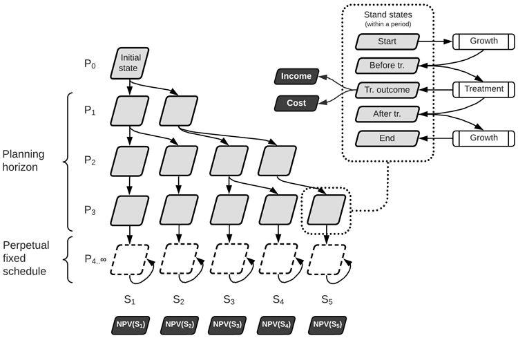
Fig. 2. Simulation procedure in GAYA 2.0. After the planning horizon, the silvicultural cycle is finalized according to the fixed schedule and the development stage. Beyond this, the fixed schedule is assumed to be applied cyclically forever. Periods are denoted P1, P2, etc., and schedules S1, S2, etc. NPV(Si) denotes the net present value of the i-th schedule.
A treatment schedule has a corresponding cash flow of the different costs and incomes for each period which are summarized as a net present value (NPV) using the preset yearly discount rate. By following a similar discounting mechanism, other non-economical values of a schedule may be calculated. For instance, the discounted carbon flow (or carbon NPV) which is valued in relation to climate change mitigation. The net present value of each schedule is calculated assuming management continuity beyond the planning horizon. This means that the possible cashflow generated after the end of the planning horizon should be discounted and integrated into the NPV. To achieve this, we assume a fixed treatment schedule to be applied indefinitely. The fixed schedules are decided based on the stand’s main species, site index, and the level of the discount rate.
The treatment schedules for a set of forest stands (or plots) and their associated NPVs are passed to the optimizer which according to user defined objective function and constraints selects the optimal schedule for each stand. Finally, user defined production tables are calculated for the optimal schedules.
3 Models
3.1 Growth models
The stand development is characterized by: (1) growth in terms of dominant height and mean diameter, and (2) natural mortality.
The models for dominant height development are species specific and based on stand’s site index (SI) and age at breast height. The user may choose between the older models [Tveite (1977) – spruce; Tveite (1976) – pine; Strand (1967) – birch] used in previous versions of GAYA, and newer updated models [Sharma et al. (2011) – spruce and pine, Eriksson et al. (1997) - birch]. In the Suppl. file S3 we show the differences in predicted dominant heights for the two sets of models.
The diameter growth models (Blingsmo 1984) are based on site index, number of trees ha–1, mean diameter, dominant height and age at breast height. The models predict 5-year increments in diameter and include an optional growth reduction factor (Braastad 1983) for stands with less than 2000 trees ha–1.
The mortality mechanism is based on: (1) normal mortality rates (Eid and Tuhus 2001), (2) density induced mortality (Hoen et al. 1998), and (3) relative diameter of dead trees (Braastad 1982). The density induced mortality is based on the Hart-Becking spacing index, where the number of removed (dead) trees corresponds to an increase in the spacing index by 1%. The density induced mortality replaces the regular one when the spacing index drops below site index specific thresholds. More details are given in Suppl. file S4.
3.2 Biometrical models
The volumes are calculated using a set of new taper functions for Norway (Hansen et al. 2023), which are based on methods from Kozak (1988) for diameter taper, and on (Gordon 1983; Stängle et al. 2016) for bark thickness. Since the taper functions are difficult to integrate analytically, we calculate the volume of a tree by numerical integration, using a fixed number of vertical slices. Obtaining accurate volumes involves dense slicing of the tree stem, but this process is computationally demanding and can create a bottleneck when running simulations. Therefore, we use a relatively low number of height slices (e.g., 20), and minimize the volume approximation errors, by finding optimal (using a heuristic approach) height locations for each species (Fig. 3).
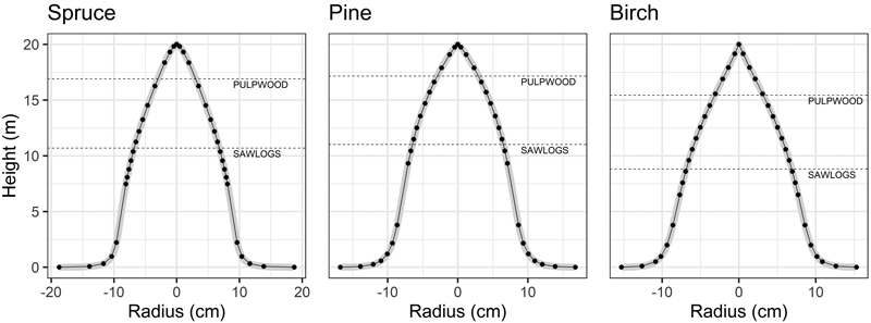
Fig. 3. GAYA 2.0 uses taper models to predict tree stem volume and its utilization with high precision. The trees in the example are 20 m in height and have a diameter at breast height of 20 cm. Pulpwood and sawlog heights correspond to minimum top diameters of 5 and 12 cm for pulpwood and sawlog, respectively. Dots mark the height location that minimize volume errors when approximating the volume of revolution of the tree stem. The tree species are Norway spruce (Picea abies), Scots pine (Pinus sylvestris), and birch (Betula pendula and B. pubescens).
The biomass (dry weight) of eight tree components are predicted with Marklund’s (1988) allometric models which have been used extensively in Norway and Sweden for many decades. The components are biomass of stem wood (SW), branches (BR), dead branches (DB), bark (SB), stump (SU), foliage (FL), fine roots (RF), and coarse roots (RC). Beyond providing values for above- and/or belowground biomass, these models play an essential role in the detailed carbon accounting module described below.
3.3 Carbon models
The carbon flow within managed forests exhibits an irregular pattern over time, which is shaped by the various treatments implemented during the silvicultural cycle. We track the carbon flow (Fig. 4) with a system of models starting with the carbon fixation in the forest biomass until it is released again into the atmosphere as CO2 through natural (i.e., decomposition) or anthropogenic (e.g., combustion) processes.
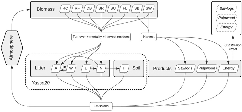
Fig. 4. The carbon cycle model in GAYA 2.0. The tree components are stem wood (SW), branches (BR), dead branches (DB), bark (SB), stump (SU), foliage (FL), fine roots (RF), and coarse roots (RC). The Yasso20 chemical compartments are celluloses (A), sugars (W), wax-like compounds (E), lignin-like compounds (N), and humus (H).
The carbon cycle starts with the sequestration in the trees’ biomass (Fig. 4). The amount of carbon stored in the trees’ biomass is based on the biomass models for the different tree components. We assume the carbon content of the biomass to be 50%.
The biomass carbon pool of the trees feeds the soil pool via litter production and decomposition and the wood products pool after it is harvested. Litter input is modeled with three different sources: (1) the normal annual turnover, (2) natural mortality, and (3) harvest residues. For each litter source, the carbon quantities are calculated as fractions of the eight biomass components of the mean tree (i.e., diameter and height), expanded by the number of trees ha–1. The turnover rates are expressed as yearly proportions of some of the tree components like needles, leaves, branches, or roots, and are derived from estimated lifetime of these components (e.g., lifetime of pine needles is approximately 3 years, thus the yearly turnover rate of 0.33). We use the values from Peltoniemi et al. (2004) and de Wit et al. (2006). The normal annual turnover is distinct from mortality and harvest residues as the generated litter is not subtracted from the biomass pool. The trees that have died during the period have their entire biomass transferred to the litter pool. The carbon transfer of the harvested trees is split between the litter and the products pool, with a certain percentage of the stem biomass being taken out from the forest as sawlogs and pulpwood (see Fig. 3) and everything else left as residue (i.e., tops, branches, roots, etc.).
The Yasso20 soil carbon model (Viskari et al. 2022) is used to simulate the process of litter decomposition. This model partitions the soil into five chemical compartments, with four of them belonging to the decomposing litter: cellulose (A), sugar (W), wax-like compounds (E), and lignin-like compounds (N) (see Fig. 4). The fifth unit is humus (H), which denotes the final stage of decomposition and is associated with the soil organic (or here simply soil) carbon pool. The chemical composition of individual tree components (by species) are the mean values from Appendix 1 in the Yasso07 manual (Liski et al. 2009). Yasso20 is published on GitHub: https://github.com/YASSOmodel/Yasso20. We have converted the original FORTRAN version of Yasso20 into C++ and seamlessly integrated the model into GAYA 2.0.
The Yasso20 model is formulated in terms of decomposition rates, with each litter compartment decomposing either into another litter compartment, humus, or released as CO2 (see Fig. 4). The carbon in the humus compartment is only emitted as CO2. The decomposition rates depend on climatic variables like the annual precipitation (mm) and mean monthly temperatures (°C).
The carbon storage in wood products is modeled by a fixed lifetime followed by a decay duration (Hoen and Solberg 1994). These parameters are estimated for 11 distinct product types, which are collapsed into three product categories: sawlogs, pulpwood, and energy (see Suppl. file S5).
Alongside the carbon flow calculation, a substitution effect is computed for the CO2 emissions reduced by utilizing wood products in place of other materials that cause higher carbon emissions. The substitution factors are from Raymer (2005) and account for reduced emission in the production process of wood materials as well as energy production using firewood, and wood products at the end of their lifetime (see Suppl. file S5).
3.4 Albedo model
Albedo can be used as a climate change mitigation tool since increasing the reflectivity of a forest stand can lead to reduced heat absorption and subsequent cooling of the surrounding area. Forest management practices such as thinning, and planting of tree species with high reflectivity can help increase albedo.
The albedo model formulated by Bright et al. (2013) is used to predict the ratio of energy reflected by a forest stand (Fig. 5). It uses two predictor variables: stand age and mean annual temperature. The model is fitted separately for spruce, pine, and birch-dominated stands since different tree species have varying reflectivity characteristics. The model is based on changes in the reflectivity of a forest stand over time due to growth and aging, and as the canopy cover closes. The temperature of the area affects the reflectivity of the surface, with warmer temperatures resulting in less snow cover and a decrease in reflectivity.
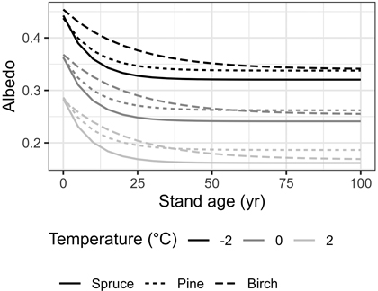
Fig. 5. GAYA 2.0 predicts forest surface albedo using the model in Bright et al. (2013). Here we illustrate albedo’s dependence on the mean annual temperature and stand age for the three species: Norway spruce (Picea abies), Scots pine (Pinus sylvestris), and birch (Betula pendula and B. pubescens).
3.5 Economic calculations
The economical component of the stand simulator predicts costs and revenues related to the stand treatments. The cash flow of a treatment schedule is aggregated as net present value (NPV) based on a preset discount rate. As the NPV should include cash flows that extend beyond the planning horizon (e.g., 100 years), a simple mechanism to predict such cash flows was set in place. First, a fixed schedule is selected based on the stand’s site index and dominant species, and the discount rate level. The schedule generated for the planning horizon is then extended with the number of periods necessary to close the silvicultural cycle. This is done by aligning the fixed schedule with the age of the stand at the end of the planning horizon. The cash flow from the extended schedule are integrated in the NPV. Lastly, under the assumption that all further forest successions will be managed under the fixed schedule, a “land value” component is calculated using the sum of the convergent geometric series, where the first term is the NPV of one fixed schedule, and the common ratio is based on the interest rate and the fixed rotation length.
The calculation of regeneration costs considers the number of stems planted and associated costs for purchase and labor. A set number of trees are assumed to regenerate naturally and cost-free (i.e., 300 stems ha–1 out of which 70% are of the main species (Hoen et al. 1998)). Some regeneration programs also include a fixed cost for soil scarification.
Basic tending costs are determined by a regression that considers the number of stems removed per hectare and the stand’s mean height, with coefficients updated periodically through an agreement between the Confederation of Norwegian Enterprise (NHO Mat og Drikke) and the United Federation of Trade Unions (Fellesforbundet) (NHO Mat og Drikke and Fellesforbundet 2022). Based on the agreement and Hoen et al. (1998) extra costs are added to account for skilled workers (10%), equipment (18%), transport (5%), terrain condition (up to 60%, varies by slope and terrain roughness), distance from road (up to 12%), and administration (40%).
The expenses associated with thinning and final harvesting activities are divided into felling and forwarding costs. The costs are based on production functions (m3 hour–1) for harvester and forwarders and corresponding machine-hour costs (EUR hour–1) (Dale et al. 1993; Dale and Stamm 1994; Eid 1998). The production functions determine the expected production for felling using factors like mean tree volume, removal percentage, number of stems ha–1 and slope, and volume ha–1, volume per load, and various distance measurements for forwarding. The machine-hour costs of felling and forwarding, based on recent data, are assessed to be 150, and 125 EUR hour–1, respectively.
The revenues are calculated based on the potential sawlogs and pulpwood quantities that results from harvests. We use the taper functions (Hansen et al. 2023) to determine the volumetry of the harvested mean tree and parameters for the minimum top diameter and length of sawlogs and pulpwood logs. This way, we determine realistic sawlogs/pulpwood proportions of the harvested wood (Fig. 3). The user provides the price for sawlogs and pulpwood in EUR m–3 by species.
4 Case study
4.1 Objectives
We showcase the capabilities of GAYA 2.0 through a case study that examined the carbon balance at a regional level. The case study aimed for the following objectives: (1) evaluate the potential for carbon sequestration under different silvicultural regimes, (2) estimate the expenses associated with different levels of carbon benefits, (3) investigate how forest management practices can adapt to accommodate increasing levels of carbon benefits, and (4) analyze the impact of improved site productivity resulting from climate warming on (1), (2), and (3). In addition, we predicted changes in forest albedo which complements the climate effects of carbon sequestration.
4.2 Materials
The study area was the Innlandet county (52 072 km2) in Norway which represents more than 40% of harvest in the country (Statistics Norway 2023) (Fig. 6). We used 2573 plots of the NNFI (Tomter et al. 2010), a large systematic sample representative for the study area. The plots were measured from 2015 through 2019. Each plot was treated as a forest stand spanning an area determined by the local sampling density. Climate data, like mean monthly temperatures and yearly precipitations were calculated by averaging readings from 47 weather stations in Innlandet over the past five years, February 2018 to February 2023 (Norwegian Meteorological Institute 2023).
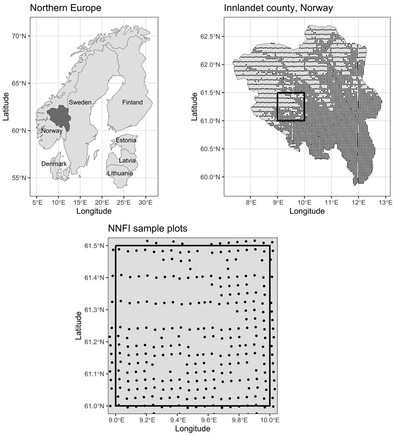
Fig. 6. The case study was conducted in Innlandet county in Norway. The approximative Norwegian National Forest Inventory (NNFI) plot locations are marked with dots. The apparent scattered plot positions are due to the random errors attached by NNFI to the coordinates when sharing plot data.
4.3 Simulations
Forest simulations were carried out on a planning horizon of 10 periods of 10 years each (100 years) and the treatments were timed at the start of each period. The prices for sawlogs and pulpwood were estimated based on official statistics from Landbruksdirektoratet (2022). These were (in EUR m–3): 62.5 – spruce, 57.5 – pine, and 40 – birch for sawlogs, and 27.5 – spruce, 25 – pine, and 30 – birch for pulp. The set of possible treatments consisted in 31 treatment definitions for tending, thinning, and final harvest methods such as shelterwood establishment and removal, seed tree establishment and removal, and clear cutting. In addition to these, 143 types of regeneration programs give natural or planted alternatives for stands with different final harvest methods, main species, site indices, vegetation types and altitude.
Scenarios of increased forest productivity were modeled by incrementing the site indexes of all plots. We considered 4 scenarios: the base scenario, with no SI increment (denoted SI+0), and three consecutive SI increments of 1 m, 2 m, and 3 m, respectively (denoted SI+1, SI+2, and SI+3) mimicking very roughly consequences of climate change. The site index increments were applied progressively from the present to the end of the planning horizon. For instance, in the SI+1 scenario, the SI increment was: 0.0 m for the present, 0.5 m 50 years from the present, and 1.0 m 100 years from the present.
4.4 Optimization problems
The simulations branched out an average of 156.2 different treatments schedules per plot, and a maximum of 1897. For each treatment schedule simulated, two variables were calculated: the monetary net present value (NPV) based on an interest rate of 3% per year, and the carbon net present value (carbon NPV) calculated as the discounted net forest carbon benefit. The same rate of discount was used for the carbon NPV (Hoen and Solberg 1994; Raymer et al. 2009). The net carbon benefit was calculated for each period as:
![]()
The litter, soil, and products carbon pools were initialized with 0at the start of the planning horizon.
To map the tradeoff curve (or optimality front) between the NPV and carbon NPV, a set of optimization problems were defined and solved with the JLP22 optimizer. First, we identified the management plans that maximized the NPV and calculated the corresponding carbon NPV. Then, by mirroring the first problem, we maximized the carbon NPV and calculated the corresponding NPV. The NPV and carbon NPV levels resulting from the two problems established the extremities of the tradeoff curve, and the range of carbon benefit levels that can be achieved through different forest management regimes. Next, the range of carbon NPV was split in nine levels, representing 10% through 90% of the range. To determine the tradeoff curve, nine additional problems were formulated, each maximizing the NPV, with the constraint that the carbon NPV should be at a set level. Another constraint, common to all optimization problems, was the fixed yearly harvest level which we choose to match the present level according to Statistics Norway (2022b). To this level we added 20% to compensate for the bark volume, tree tops and bucking leftovers which are not accounted for by Statistics Norway (Raymer et al. 2009). After the correction, the fixed yearly harvest volume was set to 5 569 200 m3.
4.5 Results
The tradeoff curves between the economic and carbon benefit are plotted in Fig. 7 – A for the different site index increments. The increased site productivity had a greater effect on the carbon NPV than it had on the NPV (Fig. 7 – C, D). In the scenarios of site index increments by 1, 2, and 3 m the NPV increased by around 2%, 3.5%, and 5%, respectively, regardless of the carbon benefit level. The carbon NPV increased by around 5.5%, 11%, and 16.5% respectively. The marginal costs of implementing different levels of carbon benefits did not vary significantly with increased productivity (Fig. 7 – B). With the highest level of carbon benefit, around 30% of the NPV would be lost. This figure, however, dropped abruptly with subsequent lower levels of carbon benefit. At 80% carbon benefit level, the marginal costs were below 10% and for 50% they were at around 2.5% of the NPV.
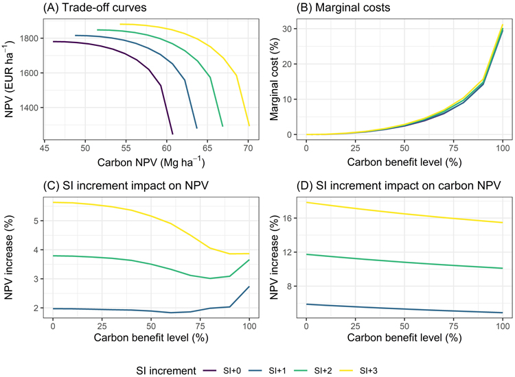
Fig. 7. GAYA 2.0 case study results. A – the trade-off curve between the net present value (NPV) and carbon NPV; B – marginal costs of different carbon benefit levels, expressed as percentage of the maximum NPV; C, D – impact of site index (SI) increments on NPV and carbon NPV, expressed as percentage increase from the base scenario SI+0.
The results suggest that it is possible to achieve a substantial level of carbon benefit by maintaining the same harvest levels and with relatively low costs. This can be achieved by adapting the forest management. In Fig. 8 we show how the prevalence of the basic silvicultural treatments varied with increasing carbon benefit levels. In general, higher carbon benefit levels were achieved by less young growth tending and more thinning. This mirrored pattern is a result of the fact that areas which “skipped” the tending were later thinned in a more mature stage. The regeneration regime shifted as expected, from the natural to planted treatments. The regeneration treatment is the initial and the main investment, thus having the biggest impact on the NPV. The prevalence of the planted regenerations, which are considerably more expensive than the natural ones, was the main factor dictating the shape of the tradeoff curve. Apart from young growth tending, the increased productivity did not have a significant effect on the treatment prevalence. More tending was performed under increased productivity. For the carbon benefit levels above 70%, twice as many tendings were performed under the SI+3 scenario compared to the base scenario.
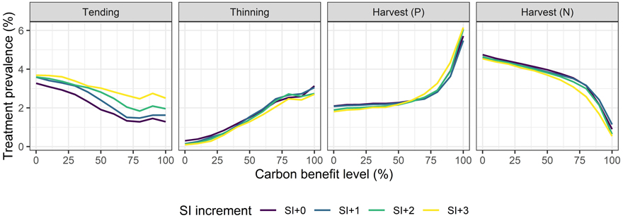
Fig. 8. GAYA 2.0 case study results. Treatment prevalence for tending, thinning, and harvest followed by planted (P), or natural (N) regeneration. The treatment prevalence is expressed as percentage of the area where the treatment was applied, averaged over the ten periods.
In Fig. 9 we show the simulated evolution of carbon changes in each pool, under optimal management regimes associated with different carbon benefit levels, as well as under scenarios of increased productivity. Regardless of the management regime or climate scenario, carbon accumulates in all pools during the entire planning horizon. It should be noted however that the litter, soil, and products pools are initialized with 0at the start of the first period, and the preexisting stocks are not considered here. The accumulation rates in the biomass pool increase up to 80 years in the future, and then decrease for the last 20 years. This is mainly due to the harvest level fixed to the present level, which in Norway are below the average growth rates of forests (Statistics Norway 2022a). As site productivity increases, we note higher change rates toward the end of the planning horizon. Higher carbon benefit levels translate in higher accumulation rates of carbon in biomass and products pools.
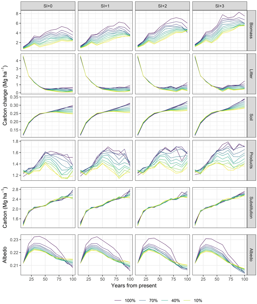
Fig. 9. GAYA 2.0 case study results. Predicted carbon changes by pool, substitution effect, and albedo over the planning horizon.
Albedo had an arched evolution, with an initial increase over 30 years followed by a subsequent decrease for the remaining planning horizon (Fig. 9). In Fig. 10 we show the evolution of the mean stand age and prevalence of the three main species proportions which are the stand variables that explain the albedo. The arched albedo trajectory is best explained by the inverse arched evolution of the mean stand age. In turn, the stand age evolution is the result of being optimal to harvest first the oldest of the stands in the early periods, as their growth has already reached a maximum. Then, due to the harvest level constrain, the stands followed an aging trend. The site index increments cause the mean stand age to increase toward the end of the horizon since with increased growth and standing wood volume, fewer stands need to be harvested to maintain the same harvest level. This translates to smaller albedo in the final periods when the site index is incremented. It should be noted however that in absolute terms, albedo did not vary a lot (i.e., ranged between 0.21 and 0.23), which is normal given the regional level averaging.
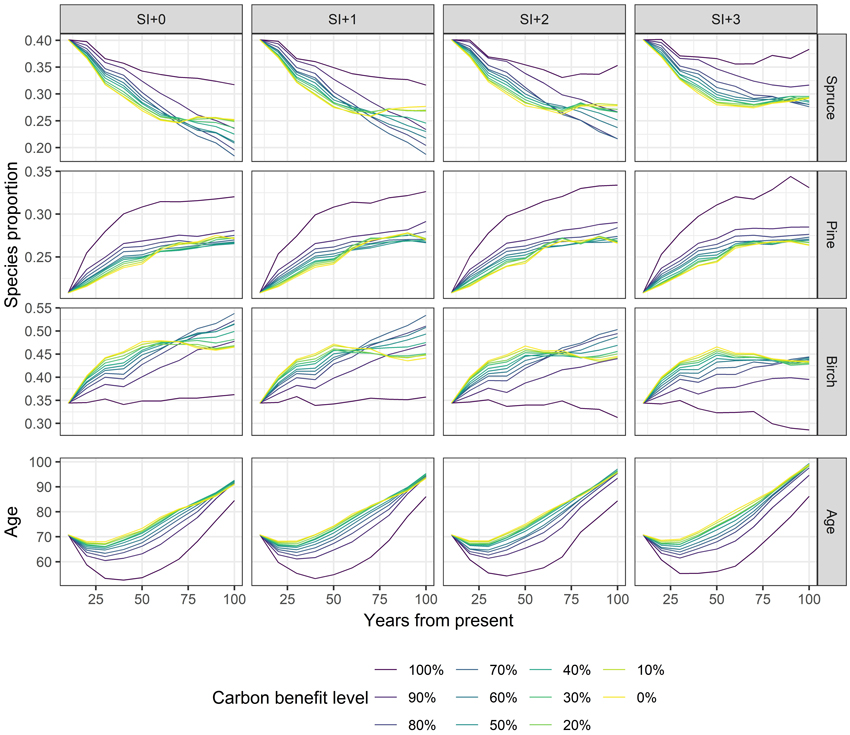
Fig. 10. GAYA 2.0 case study results. Changes in species composition and mean stand age over the planning horizon.
5 Discussion
In Norway’s forestry sector, management planning is fundamentally structured around stand-level variables. This approach is mirrored in the data collection practices during stand inventories, which focus primarily on average tree attributes and species distribution, rather than individual tree data. For this reason, stand level forest simulators (i.e., rather than individual tree level) are the pragmatic choice maximizing the range of applicability and ensuring compatibility with the industry standards. In Norway, two such models are presently used: GAYA which we have further developed, and AVVIRK-2000 (Eid and Hobbelstad 2000; Eid 2004) which is a simpler deterministic model that does not use optimization.
GAYA 2.0 has undergone a complete overhaul, now written in C++, a modern programming language using the object-oriented paradigm. The earlier version was coded in Fortran, a language that has seen diminished usage over time, thus creating barriers for maintainability and future developments. C++ allows cleaner, more maintainable code through the structured design of classes, member functions and intuitive interactions. This software has a modular, extensible architecture, parallel processing capabilities for handling large tasks, and allows users to modify an extensive set of parameters and specifications without recompiling the code.
GAYA 2.0 now includes updated models for dominant height development and tree volume estimation using taper functions. This leads to better growth predictions and more precise determinations of usable tree volume, and thus sawlogs value, by setting minimum sawlog and pulpwood log diameters.
The case study was designed to showcase some of GAYA 2.0 functionality. The scenarios demonstrate how much carbon forests can store at a regional level. Such data can be used to incorporate forests into larger carbon emissions reduction plans and policies, thereby improving their quality and effectiveness. The results also show that substantial carbon sequestration benefits can be achieved by adapting the forest management without affecting harvest levels and at relatively low costs. Our scenario model goes beyond identifying the carbon storage potential and associated costs. It also shows how forest management can be adapted to achieve specific levels of carbon benefit. The results, nonetheless, must be interpreted within the limits of the major assumptions that govern the simulations, as well as limitations in the models involved. For instance, the results of the case study suggest that larger carbon benefits may be obtained with less young growth tendings. This however may not fit well with the reality and could be a limitation of the growth models which do not explicitly handle thinning effects. It may be worthwhile to integrate such effects in future versions of GAYA (Allen Ii et al. 2020). The objectives were set for the entire region, whereas in practice, forest planning is carried out separately for individual forest estates and stands. Nonetheless, having an accurate estimate of the regional level carbon potential, regulations and incentive schemes may be designed accordingly so that individual owners can play their part. In the case study the harvests were fixed to the present. Better harvest level prognoses could be made by analyzing timeseries of past harvest levels, using forest sector models, and taking into account factory locations and capacities (Lappi and Lempinen 2014). The case study is also limited by the simple assumption on the effect of climate warming: forest productivity increases evenly across all forest types. While this is a good showcase of the types of scenarios analyses supported in GAYA 2.0, it may not be considered a fully realistic assumption.
Forest albedo is a metric that is gaining interest due to its cooling effect. However, even in cold environments like Norway, the climate effect of forest albedo is much lower than that of carbon sequestration (Rørstad 2022). Matthies and Valsta (2016) showed that including albedo with carbon storage benefits did not shorten the optimal rotation age, but it did alter the optimal species mixture by increasing the proportion of deciduous species. Nevertheless, the albedo and carbon sequestration tradeoffs may vary in high altitude or latitude regions where the forests are less productive, and the snow lasts longer.
Given the level of detail of the stand level simulations, GAYA 2.0 gives multiple opportunities to perform scenario analyses of many kinds. Previous versions of GAYA were successfully used to analyze the economic impact of biodiversity protection (Bergseng et al. 2012) and the impact of root rot risk on the optimal harvest time (Aza et al. 2021). Integrating more features describing biodiversity and different risk models (e.g., bark beetle, root rot, windthrow) in GAYA is an important future direction of development. In the risk mitigation context, GAYA may also be used to assess the value of information or perform cost-plus-loss analyses (Eid et al. 2004). With renewed interest and promoting of selective cutting it could be useful to add single tree growth models or diameter distribution models, e.g., Gobakken et al. (2008), in future versions of GAYA. Presently, however, no appropriate single tree growth models covering the entire Norwegian forest area exist. The accuracy of simulations is dependent on the quality of the underlying models and sensitivity to assumptions. To maintain high quality simulations, models need to be regularly updated, along with the parameters that determine costs, prices, and other important assumptions.
6 Conclusion
GAYA 2.0 is a valuable tool for performing scenario analyses of different kinds for forest management in Norway. It can assist in answering questions related to the future carbon sequestration potential of forests under different management regimes, the expected net present value of such regimes, and possible impacts of climate change. The simulator has been successfully used in a case study to map the tradeoff between the carbon benefit and net present value when harvest levels were kept constant at their present values. GAYA 2.0 has been updated and modernized from its previous version with increased attention to forest carbon and energy fluxes.
Declaration of openness of research materials, data, and code
Parts of the GAYA 2.0 code could be shared upon request. The possibility to share the entire code with the public via a GitHub repository is currently analyzed. The plot data used in the case study belongs to the Norwegian National Forest Inventory.
Authors’ contributions
Victor Strîmbu: Developed GAYA 2.0. Performed the case study and analyzed the results. Wrote the manuscript.
Tron Eid: Provided expertise on the biological and economic assumptions in GAYA 2.0. Assisted in testing GAYA 2.0. Revised the manuscript.
Terje Gobakken: Assisted throughout the implementation process of GAYA 2.0. Formulated the research questions for the case study. Revised the manuscript.
Funding
This study was funded by the Research Council of Norway in the project ForestPotential: “Changing forest area and forest productivity – climatic and human causes, effects, monitoring options, and climate mitigation potential” (project no. 281066), and CSFN: “Climate Smart Forestry Norway” (project no. 302701).
References
Allen Ii MG, Antón-Fernández C, Astrup R (2020) A stand-level growth and yield model for thinned and unthinned managed Norway spruce forests in Norway. Scand J Forest Res 35: 238–251. https://doi.org/10.1080/02827581.2020.1773525.
Aza A, Kangas A, Gobakken T, Kallio AMI (2021) Effect of root and butt rot uncertainty on optimal harvest schedules and expected incomes at the stand level. Ann For Sci 78, article id 70. https://doi.org/10.1007/s13595-021-01072-1.
Bergseng E, Ask JA, Framstad E, Gobakken T, Solberg B, Hoen HF (2012) Biodiversity protection and economics in long term boreal forest management – a detailed case for the valuation of protection measures. Forest Policy Econ 15: 12–21. https://doi.org/10.1016/j.forpol.2011.11.002.
Blingsmo KR (1984) Diametertilvekstfunksjoner for bjørk-, furu- og granbestand. [Diameter increment functions for stands of birch, Scots pine and Norway spruce]. Meddr norske skogforsVes 7/84, Norwegian Forest Research Institute. https://urn.nb.no/URN:NBN:no-nb_digibok_2013012108152.
Braastad H (1982) Naturlig avgang i granbestand. [Natural mortality in Picea abies stands]. Meddr norske skogforsVes 12/82, Norwegian Forest Research Institute. https://urn.nb.no/URN:NBN:no-nb_digibok_2013121908193.
Braastad H (1983) Produksjonsnivået i glissen og ujamn granskog. [Yield level in Picea abies stands with low initial density and irregular spacing]. Meddr norske skogforsVes 7/83, Norwegian Forest Research Institute. https://urn.nb.no/URN:NBN:no-nb_digibok_2013080508381.
Bright RM, Astrup R, Strømman AH (2013) Empirical models of monthly and annual albedo in managed boreal forests of interior Norway. Climatic Change 120: 183–196. https://doi.org/10.1007/s10584-013-0789-1.
Dale Ø, Stamm J (1994) Grunnlagsdata for kostnadsanalyse av alternative hogstformer. [Base data for harvesting cost analysis on alternative silvicultural methods]. Meddr norske skogforsVes 7/94, Norwegian Forest Research Institute. https://urn.nb.no/URN:NBN:no-nb_digibok_2013120608256.
Dale Ø, Kjøstelsen L, Aamodt HE (1993) Mekaniserte lukkede hogster. [Mechanized selective cuttings], chapter from Flerbruksrettet driftsteknikk. [Forest operations for multiple use]. Meddr norske skogforsVes 20/93: 3–23, Norwegian Forest Research Institute. https://urn.nb.no/URN:NBN:no-nb_digibok_2009092900072.
de Wit HA, Palosuo T, Hylen G, Liski J (2006) A carbon budget of forest biomass and soils in southeast Norway calculated using a widely applicable method. For Ecol Manag 225: 15–26. https://doi.org/10.1016/j.foreco.2005.12.023.
Eid T (1998) Langsiktige prognoser og bruk av prestasjonsfunksjoner for å estimere kostnader ved mekanisert drift. [Long-term prognoses and the use of productivity functions for cost estimation in mechanised harvesting and forwarding]. Meddr norske skogforsVes 7/98, Norwegian Forest Research Institute. https://urn.nb.no/URN:NBN:no-nb_digibok_2010042106083.
Eid T (2004) Testing a large-scale forestry scenario model by means of successive inventories on a forest property. Silva Fenn 38: 305–317. https://doi.org/10.14214/sf.418.
Eid T, Hobbelstad K (2000) AVVIRK-2000: a large-scale forestry scenario model for long-term investment, income and harvest analyses. Scand J Forest Res 15: 472–482. https://doi.org/10.1080/028275800750172736.
Eid T, Tuhus E (2001) Models for individual tree mortality in Norway. For Ecol Manag 154: 69–84. https://doi.org/10.1016/S0378-1127(00)00634-4.
Eid T, Gobakken T, Næsset E (2004) Comparing stand inventories for large areas based on photo-interpretation and laser scanning by means of cost-plus-loss analyses. Scand J Forest Res 19: 512–523. https://doi.org/10.1080/02827580410019463.
Eriksson H, Johansson U, Kiviste A (1997) A site‐index model for pure and mixed stands of Betula pendula and Betula pubescens in Sweden. Scand J Forest Res 12: 149–156. https://doi.org/10.1080/02827589709355396.
EU Comission (2021) New EU forest strategy for 2030. https://eur-lex.europa.eu/legal-content/EN/ALL/?uri=COM:2021:572:FIN. Accessed 30 March 2023.
Fankhauser S, Smith SM, Allen M, Axelsson K, Hale T, Hepburn C, Kendall JM, Khosla R, Lezaun J, Mitchell-Larson E, Obersteiner M, Rajamani L, Rickaby R, Seddon N, Wetzer T (2022) The meaning of net zero and how to get it right. Nat Clim Change 12: 15–21. https://doi.org/10.1038/s41558-021-01245-w.
Free Software Fundation Inc. (2020) MinGW-w64.
Gobakken T, Lexerød NL, Eid T (2008) T: a forest simulator for bioeconomic analyses based on models for individual trees. Scand J Forest Res 23: 250–265. https://doi.org/10.1080/02827580802050722.
Gordon A (1983) Estimating bark thickness of Pinus radiata. NZ J For Sci 13: 340–348. https://www.scionresearch.com/__data/assets/pdf_file/0006/59568/NZJFS1331983GORDON340_353.pdf.
Government of Norway (2022) Norway’s new climate target: emissions to be cut by at least 55%. https://www.regjeringen.no/en/aktuelt/norways-new-climate-target-emissions-to-be-cut-by-at-least-55-/id2944876/. Accessed 16 February 2023.
Hale T, Smith SM, Black R, Cullen K, Fay B, Lang J, Mahmood S (2022) Assessing the rapidly-emerging landscape of net zero targets. Clim Policy 22: 18–29. https://doi.org/10.1080/14693062.2021.2013155.
Hansen E, Rahlf J, Astrup R, Gobakken T (2023) Taper and volume models for spruce, pine, and birch in Norway. Scand J Forest Res. https://doi.org/10.1080/02827581.2023.2243821.
Hoen HF, Eid T (1990) En modell for analyse av behandlingsalternativer for en skog ved bestandssimulering og lineær programmering. [A model for analyses of treatment strategies for a forest applying stand simulations and linear programming]. Meddr norske skogforsVes 9/90: 1–35, Norwegian Forest Research Institute. https://urn.nb.no/URN:NBN:no-nb_digibok_2009072300129.
Hoen HF, Gobakken T (1997) Brukermanual for bestandssimulatoren GAYA V1.20. [User manual for forest stand simulator GAYA V1.20]. [manuscript]. Institutt for Skogfag, Norges Landbrukshøgskole.
Hoen HF, Solberg B (1994) Potential and economic efficiency of carbon sequestration in forest biomass through silvicultural management. Forest Sci 40: 429–451. https://doi.org/10.1093/forestscience/40.3.429.
Hoen HF, Solberg B (1997) CO2‐taxing, timber rotations, and market implications. Crit Rev Env Sci Tec 27: 151–162. https://doi.org/10.1080/10643389709388516.
Hoen HF, Eid T, Veisten K, Økseter P (1998) Økonomiske konsekvenser av tiltak for et bærekraftig skogbruk. Forutsetninger og metodebeskrivelse. [Economic consequences of means for sustainable forest management – description of methodology and data]. Meddr norske skogforsVes 6/98: 1–48, Norwegian Forest Research Institute. https://urn.nb.no/URN:NBN:no-nb_digibok_2009092301036.
Kozak A (1988) A variable-exponent taper equation. Can J Forest Res 18: 1363–1368. https://doi.org/10.1139/x88-213.
Landbruksdirektoratet (2022) Tømmeravvirkning og -priser. [Timber logging and prices]. https://www.landbruksdirektoratet.no/nb/statistikk-og-utviklingstrekk/utviklingstrekk-i-skogbruket/tommeravvirkning-og-priser. Accessed 5 February 2023.
Lappi J (2003) J-user’s guide, version 0.7.8. [manuscript]. Finnish Forest Research Institute, Suonenjoki.
Lappi J (2022) Jlp22 GitHUB repository. https://github.com/juhalappi/Jlp22. Accessed 30 March 2023.
Lappi J, Lempinen R (2014) A linear programming algorithm and software for forest-level planning problems including factories. Scand J Forest Res 29: 178–184. https://doi.org/10.1080/02827581.2014.886714.
Liski J, Tuomi M, Rasinmäki J (2009) Yasso07 user-interface manual. [manuscript]. Finnish Environment Institute.
Marklund LG (1988) Biomass functions for pine, spruce and birch in Sweden. Report 45, Swedish University of Agricultural Sciences, Department of Forest Survey.
Matthies BD, Valsta LT (2016) Optimal forest species mixture with carbon storage and albedo effect for climate change mitigation. Ecol Econ 123: 95–105. https://doi.org/10.1016/j.ecolecon.2016.01.004.
NHO Mat og Drikke and Fellesforbundet (2022) Overenskomst for Naturbruk 2022–2024 mellom Næringslivets Hovedorganisasjon og NHO Mat og Drikke på den ene side og Landsorganisasjonen i Norge og Fellesforbundet på den annen. [Agreement for Natural Resources 2022–2024 between the Confederation of Norwegian Enterprise and NHO Food and Drink on one side and the Norwegian Confederation of Trade Unions and the United Federation on the other]. https://www.fellesforbundet.no/globalassets/lonn-og-tariffsaker/tariffavtaler/overenskomster-2022-2024/33244-naturbruk-overenskomst-2022-2024-nett.pdf. Accessed 30 March 2023.
Norwegian Meteorological Institute (2023) SeNorge. https://www.senorge.no/. Accessed 16 February 2023.
OpenMP Architecture Review Board (2015) The OpenMP API specification for parallel programming.
Oracle Corporation (2018) NetBeans IDE developement version.
Pachauri RK, Allen MR, Barros VR, Broome J, Cramer W, Christ R, Church JA, Clarke L, Dahe Q, Dasgupta P, Dubash NK, Edenhofer O, Elgizouli I, Field CB, Forster P, Friedlingstein P, Fuglestvedt J, Gomez-Echeverri L, Hallegatte S, Hegerl G, Howden M, Jiang K, Jimenez Cisneroz B, Kattsov V, Lee H, Mach KJ, Marotzke J, Mastrandrea MD, Meyer L, Minx J, Mulugetta Y, O’Brien K, Oppenheimer M, Pereira JJ, Pichs-Madruga R, Plattner G-K, Pörtner H-O, Power SB, Preston B, Ravindranath NH, Reisinger A, Riahi K, Rusticucci M, Scholes R, Seyboth K, Sokona Y, Stavins R, Stocker TF, Tschakert P, van Vuuren D, van Ypserle J-P (2014) Climate change 2014: synthesis report. Contribution of Working Groups I, II and III to the Fifth Assessment Report of the Intergovernmental Panel on Climate Change. IPCC. https://epic.awi.de/id/eprint/37530/.
PEFC (2022) Ny Norsk PEFC Skogstandard. [New Norwegian PEFC Forest Standard]. https://pefc.no/nyheter/ny-norsk-pefc-skogstandard-godkjent. Accessed 16 February 2023
Peltoniemi M, Mäkipää R, Liski J, Tamminen P (2004) Changes in soil carbon with stand age – an evaluation of a modelling method with empirical data. Glob Change Biol 10: 2078–2091. https://doi.org/10.1111/j.1365-2486.2004.00881.x.
Raymer AK, Gobakken T, Solberg B, Hoen HF, Bergseng E (2009) A forest optimisation model including carbon flows: application to a forest in Norway. For Ecol Manag 258: 579–589. https://doi.org/10.1016/j.foreco.2009.04.036.
Raymer AKP (2005) Modelling and analysing climate gas impacts of forest management. PhD thesis 11, Department of Ecology and Natural Resource Management, Norwegian University of Life Sciences. https://depotbiblioteket.no/cgi-bin/m2?tnr=326746.
Rørstad PK (2022) Payment for CO2 sequestration affects the Faustmann rotation period in Norway more than albedo payment does. Ecol Econ 199: 1:14. https://doi.org/10.1016/j.ecolecon.2022.107492.
Sharma RP, Brunner A, Eid T, Øyen B-H (2011) Modelling dominant height growth from national forest inventory individual tree data with short time series and large age errors. For Ecol Manag 262: 2162–2175. https://doi.org/10.1016/j.foreco.2011.07.037.
Smith HB, Vaughan NE, Forster J (2022) Long-term national climate strategies bet on forests and soils to reach net-zero. Commun Earth Environ 3, article id 305. https://doi.org/10.1038/s43247-022-00636-x.
Stängle SM, Weiskittel AR, Dormann CF, Brüchert F (2016) Measurement and prediction of bark thickness in Picea abies: assessment of accuracy, precision, and sample size requirements. Can J Forest Res 46: 39–47. https://doi.org/10.1139/cjfr-2015-0263.
Statistics Norway (2022a) Landsskogtakseringen. [National Forest Inventory]. https://www.ssb.no/jord-skog-jakt-og-fiskeri/skogbruk/statistikk/landsskogtakseringen. Accessed 16 February 2023
Statistics Norway (2022b) Tabellen 11712: avvirkning av industrivirke for salg, etter treslag (1000 m3) (F), foreløpige tall 2017–2022. [Harvesting of industrial timber for sale, by tree species (1000 m³) (F), preliminary figures 2017–2022]. https://www.ssb.no/statbank/table/11712. Accessed 16 February 2023
Statistics Norway (2023) Skogavvirkning for salg. [Timber logging for sale]. https://www.ssb.no/jord-skog-jakt-og-fiskeri/skogbruk/statistikk/skogavvirkning-for-salg. Accessed 16 February 2023
Strand L (1967) Produksjonstabeller for bjork. [Yield tables for birch]. Kap IX, Hoydekurver for bjork. [Site index curves for birch]. Meddr norske skogforsVes 22: 265–365, Norwegian Forest Research Institute. https://urn.nb.no/URN:NBN:no-nb_digibok_2017080748051.
Tomter SM, Hylen G, Nilsen J-E (2010) Development of Norway’s National Forest Inventory. In: Tomppo E, Gschwantner T, Lawrence M, McRoberts RE (eds) National forest inventories – pathways for common reporting. Springer, pp 411–424. https://doi.org/10.1007/978-90-481-3233-1.
Tveite B (1976) Bonitetskurver for furu. [Site-index curves for pine]. Internal report, unpublished. Norsk Institutt for Skogforskning.
Tveite B (1977) Bonitetskurver for gran. [Site-index curves for spruce]. Meddr norske skogforsVes 33/77, Norwegian Forest Research Institute. https://urn.nb.no/URN:NBN:no-nb_digibok_2012112906103.
Viskari T, Pusa J, Fer I, Repo A, Vira J, Liski J (2022) Calibrating the soil organic carbon model Yasso20 with multiple datasets. Geosci Model Dev 15: 1735–1752. https://doi.org/10.5194/gmd-15-1735-2022.
Total of 58 references.
