Eetu Kotivuori  ,
Lauri Korhonen,
Petteri Packalen
,
Lauri Korhonen,
Petteri Packalen
Nationwide airborne laser scanning based models for volume, biomass and dominant height in Finland
Kotivuori E., Korhonen L., Packalen P. (2016). Nationwide airborne laser scanning based models for volume, biomass and dominant height in Finland. Silva Fennica vol. 50 no. 4 article id 1567. https://doi.org/10.14214/sf.1567
Highlights
- Pooled data from nine inventory projects in Finland were used to create nationwide laser-based regression models for dominant height, volume and biomass
- Volume and biomass models provided regionally different means than real means, but for dominant height the mean difference was small
- The accuracy of general volume predictions was nevertheless comparable to relascope-based field inventory by compartments.
Abstract
The aim of this study was to examine how well stem volume, above-ground biomass and dominant height can be predicted using nationwide airborne laser scanning (ALS) based regression models. The study material consisted of nine practical ALS inventory projects taken from different parts of Finland. We used field sample plots and airborne laser scanning data to create nationwide and regional models for each response variable. The final models had one or two ALS predictors, which were chosen based on the root mean square error (RMSE), and cross-validated. Finally, we tested how much predictions would improve if the nationwide models were calibrated with a small number of regional sample plots. Although forest structures differ among different parts of Finland, the nationwide volume and biomass models performed quite well (leave-inventory-area-out RMSE 22.3% to 33.8%, mean difference [MD] –13.8% to 18.7%) compared with regional models (leave-plot-out RMSE 20.2% to 26.8%). However, the nationwide dominant height model (RMSE 5.4% to 7.7%, MD –2.0% to 2.8%, with the exception of the Tornio region – RMSE 11.4%, MD –9.1%) performed nearly as well as the regional models (RMSE 5.2% to 6.7%). The results show that the nationwide volume and biomass models provided different means than real means at regional level, because forest structure and ALS device have a considerable effect on the predictions. Large MDs appeared especially in northern Finland. Local calibration decreased the MD and RMSE of volume and biomass models. However, the nationwide dominant height model did not benefit much from calibration.
Keywords
forest inventory;
LIDAR;
regression analysis;
remote sensing;
calibration;
area-based approach;
mixed-effect models
-
Kotivuori,
University of Eastern Finland, School of Forest Sciences, P.O. Box 111, FI-80101 Joensuu, Finland
E-mail
eetu.kotivuori@uef.fi
- Korhonen, University of Eastern Finland, School of Forest Sciences, P.O. Box 111, FI-80101 Joensuu, Finland E-mail lauri.korhonen@uef.fi
- Packalen, University of Eastern Finland, School of Forest Sciences, P.O. Box 111, FI-80101 Joensuu, Finland E-mail petteri.packalen@uef.fi
Received 12 February 2016 Accepted 27 June 2016 Published 8 July 2016
Views 131297
Available at https://doi.org/10.14214/sf.1567 | Download PDF

1 Introduction
Airborne laser scanning (ALS) and especially the area-based approach (ABA) for predicting forest inventory attributes have been widely studied and utilized in forest inventories (Næsset 2014; Maltamo and Packalen 2014). In the area-based approach, plot level metrics are computed from an ALS echo cloud. Empirical models are fitted using ALS metrics as independent variables, and field measurements of sample plots as dependent variables (Næsset 2002). These models are used for the prediction of stand attributes for a whole region. In other words, ALS data contains information about horizontal and vertical echo distributions, which can be used to describe the forest structure in an area (Vauhkonen et al. 2014). However, sample plot field measurements are time consuming and expensive. For this reason, it is tempting to create models for areas larger than a typical inventory project, or to utilize sample plots from earlier inventory areas. Unfortunately, if the inventory area is so large that several ALS data acquisitions are needed or the forest structure varies within the area, the large-area model predictions have different means than real means at regional level and are less accurate than models fitted separately for each region or ALS campaign (Næsset and Gobakken 2008; Næsset 2009). However, calibration of existing ALS-based models could be used to mitigate the problem.
Not many studies have been conducted on this topic. Næsset et al. (2005) approached the problem by using two different inventory areas. They compared a general model composed of two regions fitted by ordinary least squares (OLS), seemingly unrelated (SUR), and partial least squares (PLS) regression methods, to regional models fitted by OLS estimation. According to Næsset et al. (2005), it could be possible to utilize existing sample plots in new inventory projects, if the relationships between the ALS and field data remain relatively stable. Also, it should be confirmed that the previously measured plots sufficiently represent forests in the new area. However, in their study there were no significant differences between the regression methods. Moreover, because of the straightforward interpretation of the results and availability of effective metric selection of the models, the authors recommended that OLS-regression should be preferred when fitting general models (Næsset et al. 2005). In turn, Næsset (2007) evaluated results of an operational ALS-based stand level forest inventory, combining sample plots from two districts. They used stepwise OLS estimation with small sample plots (250 m2) as a training dataset and large sample plots (1000 m2) as validation stands. The results showed that there were no significant effects related to district in most of the used models. Also, no large mean differences were detected. However, the areas were located close to each other (50 km).
Suvanto and Maltamo (2010) studied the subject using weighted OLS estimation, known as mixed estimation. ALS and sample plot data were collected from the areas of Matalansalo and Juuka, located 120 kilometers apart in eastern Finland. The study compared OLS estimation using a merged dataset with calibration by mixed estimation and local models. Model comparisons were done using five simulated estimation procedures: 1. merged dataset, 2.–3. mixed estimations, and 4.–5. local models. In the mixed estimation, Juuka plots (n = 10–212) were used as a sample from the target population and Matalansalo plots as auxiliary data. Local models were fitted using only the Juuka plots and either predetermined variables or independent variable selection. According to the results of the study, mixed estimation offered improved predictions compared to the OLS estimated general model. However, it was possible to obtain equally accurate predictions of stem volume and basal area by building local models based on 40–50 plots, instead of using the auxiliary data taken from Matalansalo (Suvanto and Maltamo 2010). In turn, Breidenbach et al. (2008) examined the subject with mixed-effect models. They found that the prediction of stand attributes with two separate inventory areas was more accurate with mixed-effect models than with models having only fixed effects. Breidenbach et al. (2008) showed that general models with mixed-effects were able to describe separate datasets with great success. According to Breidenbach et al. (2008), mixed-effect models are also easy to calibrate to a new inventory area with a small number of sample plots.
All of the above mentioned studies compared only two regions. However, Næsset and Gobakken (2008) used 10 different areas for the prediction of above-ground biomass across the regions. Næsset and Gobakken used three-phased multiple regression analysis, where they: 1) tried to find the best ALS-variables to explain biomass; 2) tested the stability of models with different plot combinations; and 3) assessed the effects of ALS device, geographical region and forest type. The results showed that biomass models with sensor, region and forest type dummy variables explained the variability of above-ground biomass across the regions with relatively good levels of accuracy (R2 = 88%). Subjective assessment indicated that the differences between the areas were probably caused by the different geographical regions, rather than different ALS devices. Because of these geographical effects, they recommend that plots should be distributed over the entire area in ALS-based regional or national biomass monitoring.
These studies indicate that modelling separate geographical areas using the same ALS-based models is affected by variation in forest structure, which can be described, for example, with biomass, stem number, basal area, canopy height and the density of trees (Delang and Li 2013). In Finland, forest structure is affected by geographical gradients, especially in a north-south direction. This can be seen as a variation in e.g. volume between northern and southern parts of Finland. According to the Finnish Statistical Yearbook of Forestry (2014), southern Finland has an average growing stock of 139 m3 ha–1, while in north the corresponding value is only 81 m3 ha–1. The main reason for the different forest structures is that the productivity per year is almost one cubic meter (m3 ha–1) lower in northern than in southern Finland (Metsäntutkimuslaitos 2014).
Another reason that makes it difficult to utilize nationwide ALS based models is non-uniform ALS data. The reasons for this are different ALS devices, flying and scanning parameters, and data collection dates. Differences between ALS devices can be noted as differences in canopy height distributions (Næsset 2005) or density metrics (Næsset 2009). These differences can be caused by larger pulse energy and peak power, which lead to increasing penetration into the canopy (Næsset 2005; Hopkinson 2007). According to Næsset (2009), higher pulse repetition frequencies (PRFs) cause upward shifts in the canopy height distributions. Higher flight altitude decreases the proportion of multiple echoes and can also lead to decreased penetration (Næsset 2004; Næsset 2009). However, the flight altitude does not usually have a major influence on the predicted forest attributes, because regression compensates for these differences (Næsset 2004; Næsset 2009). In addition, combination of leaf-off and leaf-on (or partial leaf-on) datasets is not recommended, because the values of canopy density metrics are significantly reduced when using leaf-off data (Næsset 2005; Villikka et al. 2012). The reduction of canopy density also increases the accuracy of predicted stand properties (Næsset 2005; Villikka et al. 2012).
Our main objective was to study how accurately the stem volume, biomass and dominant height can be predicted using a nationwide, ALS-based regression model. Although such model predictions may have different mean than the real value, they can still be useful in situations where ALS data are available, but field data are lacking. We fitted both nationwide and regional models using OLS-estimation based on data from nine inventory areas, and validated the results by means of cross-validation. The accuracy of different models was compared using root mean square error (RMSE) and a measure of mean difference (MD). Finally, we tested how much predictions would improve if the nationwide models were calibrated using a small number of regional sample plots. The calibration was performed using mixed-effect models.
2 Materials and methods
The study material consisted of nine Finnish Forest Centre inventory projects situated in various parts of Finland (Fig. 1). The field sample plots and ALS data from each inventory area were used to construct nationwide and regional models. ALS data were provided by Blom Kartta and TerraTec, and the sample plots were obtained from the Finnish Forest Centre. However, ALS data is freely available on the web site of the National Land Survey of Finland. Regionally, the inventory areas of Kolari, Tornio and Ranua located in northern Finland have considerably poorer growth conditions than the other areas.
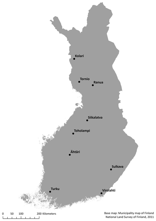
Fig. 1. Map of the inventory areas.
2.1 Field measurements
There were some differences in the field measurement procedures because of the different contractors involved. The inventory areas of Siikalatva, Toholampi, Sulkava, Virolahti and Turku were measured using the official field guide of the Finnish Forestry Centre (Suomen Metsäkeskus 2014). Ähtäri was measured using the guide of the National Forest Inventory and the Finnish Forest Centre (Metla and Suomen Metsäkeskus 2013). Kolari was measured using the field guide of TerraTec (Ratilainen 2011), and Tornio and Ranua were measured using the general field guide provided for Blom Kartta’s subcontractors (Blom Kartta Oy 2012). The differences seen were related to the plot placement and size, the minimum tree diameter at breast height, and tree height measurements.
In Ähtäri, the sample plots were placed systematically in the whole inventory area with L-shape clusters, while in the other inventory areas the plots were placed using random or systematic stratified cluster sampling. Because of the sampling method, twice as many plots were measured in Ähtäri compared with other regions. In addition, there were four different plot sizes and differing tree diameter thresholds for tally trees. In general, in mature stands the tally trees were measured using plot radii of either 9, 12.62 or 12.65 m, and in seedling stands using a plot radius of 5.65 m. In order to harmonize the data, all trees with a diameter < 5 cm were removed. Moreover, the height measurements varied among the measurement protocols. In the field measurements of Blom Kartta and TerraTec the heights of all of the tally trees were measured, but in the other inventory areas only heights of the sample trees were measured. Finally, all plots placed in seedling stands were removed due to their small mean diameter. In the end, there were about 1200 sample plots from the inventory area of Ähtäri and 500–700 plots from the other areas, giving a total of 6230 plots (Table 1).
| Table 1. Field measurement dates, number of sample plots, observed mean volume, mean biomass and mean dominant height in each inventory area. Inventory areas are ordered from north to south. | |||||
| Inventory area | Time window | Number of sample plots | Volume (m3 ha–1) | Biomass (t ha–1) | Dominant height (m) |
| Kolari | 29.05.2013 – 07.10.2013 | 534 | 100.9 | 56.3 | 13.9 |
| Tornio | 28.05.2013 – 07.11.2013 | 596 | 97.2 | 57.3 | 12.7 |
| Ranua | 28.05.2012 – 24.10.2012 | 613 | 98.3 | 55.9 | 12.9 |
| Siikalatva | 20.06.2013 – 18.10.2013 | 657 | 118.0 | 64.4 | 15.6 |
| Toholampi | 26.07.2012 – 29.10.2012 | 587 | 102.8 | 55.8 | 14.7 |
| Ähtäri | 23.05.2013 – 25.10.2013 | 1233 | 139.7 | 73.9 | 16.8 |
| Sulkava | 01.07.2011 – 04.01.2012 | 570 | 173.4 | 90.3 | 18.6 |
| Virolahti | 13.05.2013 – 15.11.2013 | 724 | 179.4 | 93.5 | 17.8 |
| Turku | 23.04.2012 – 14.11.2012 | 716 | 180.9 | 93.6 | 18.8 |
Field data were used to calculate the stem volume, above-ground biomass and dominant height. The means of these plot level attributes for all of the inventory areas are presented in Table 1. In the table, the means differ significantly between regions, especially in a north-south direction. For example, basal area is about 15% smaller, dominant height over 20% smaller, and above-ground biomass about 30% smaller on average in the north than in the south. A summary of volume, biomass and dominant height by tree species is presented in Table 2 for all of the sample plots.
| Table 2. Summary of distribution values for volume, biomass and dominant height by tree species for all of the sample plots in the modelling dataset. | ||||||
| Minimum | 1. Quartile | Median | Mean | 3. Quartile | Maximum | |
| Volume (m³ ha–1) | ||||||
| Pine | 0.0 | 8.3 | 54.2 | 71.8 | 110.5 | 572.4 |
| Spruce | 0.0 | 0.0 | 3.7 | 40.5 | 41.1 | 839.3 |
| Birch | 0.0 | 0.0 | 5.0 | 21.3 | 25.2 | 406.4 |
| Other d.t.* | 0.0 | 0.0 | 0.0 | 1.3 | 0.0 | 581.5 |
| Total | 3.0 | 63.1 | 114.1 | 134.9 | 184.3 | 915.5 |
| Biomass (t ha–1) | ||||||
| Pine | 0.0 | 4.7 | 28.8 | 36.7 | 57.3 | 244.4 |
| Spruce | 0.0 | 0.0 | 2.7 | 22.8 | 26.4 | 366.1 |
| Birch | 0.0 | 0.0 | 2.8 | 12.2 | 14.6 | 206.6 |
| Other d.t.* | 0.0 | 0.0 | 0.0 | 0.7 | 0.0 | 302.5 |
| Total | 1.8 | 36.0 | 62.9 | 72.4 | 98.6 | 409.1 |
| Dominant height (m) | ||||||
| Total | 3.9 | 12.1 | 15.9 | 16.0 | 19.5 | 32.9 |
| * Other deciduous trees | ||||||
2.2 Plot attributes
The volume of trees was calculated using Laasasenaho’s models with two predictors (Laasasenaho 1982):
![]()
![]()
where outcome v is the volume in liters, d is the diameter at beast height in centimeters, and h is the tree height in meters. The volume of other deciduous trees was calculated using the volume model of birch. Finally, tree level volumes were summed on a plot level and weighted to a per hectare unit by the plot area (m3 ha–1).
The above-ground biomass was calculated using Repola’s tree level biomass models (Repola 2008, 2009):


where agb is the above-ground biomass in kilograms, dk is the stump height diameter in centimeters (dk = 2 + 1.25d), h is the tree height in meters, and Se2 is the unbiased estimator of residual variance. The biomass models included a natural logarithm transformation which caused a bias which we accounted for using a bias correction of nonlinear prediction (Lappi 1993). Finally, the tree level biomasses were summed on a plot level and weighted to a per hectare unit (t ha–1). The dominant height was determined as the mean height of the 100 trees with the largest diameter at breast height per hectare (Kangas et al. 2011).
2.3 ALS data
The ALS devices and scanning parameters used in the different inventory areas are presented in Table 3. The data acquisitions were performed in 2011–2013, between June and August. Two different sensor models were used (Leica ALS 70-Ha and Optech ALTM Gemini), and four different sensor units (denoted A–D). Table 3 shows that the flight altitude varied between 1730–2000 meters, and the pulse repetition frequency between 50 000–71 800 hz. The half scan angle was 15 degrees in the inventory areas of Kolari, Siikalatva and Sulkava, and 20 degrees elsewhere. All of the areas were scanned using a one-pulse-in-the-air scanner mode. A Digital Terrain Model (DTM) was constructed by first classifying the echoes as ground and non-ground according to the approach described by Axelsson (2000). A raster DTM was then obtained by interpolation using Delaunay triangulation. The above-ground heights (dZ) for ALS echoes were calculated by differencing their elevations above the ellipsoid from corresponding DTM elevations.
| Table 3. The sensor models, sensor units (A–D), scanning time windows, flying altitudes, pulse repetition frequencies (PRF), half scan angles, and mean pulse density for each project. | |||||||
| Inventory area | Sensor model | Sensor unit | Time window | Altitude (m) | PRF (hz) | Half scan angle (degrees) | Pulse density (pl/m2) |
| Kolari | Optech ALTM Gemini | B | 07.06. – 06.08.2013 | 1950 | 50 000 | 15 | 0.6 |
| Tornio | Leica ALS 70-HA | C | 13.06. – 04.08.2013 | 1950 | 71 000 | 20 | 0.5 |
| Ranua | Optech ALTM Gemini | A | 04.07. – 24.08.2012 | 1750 | 70 000 | 20 | 1.0 |
| Siikalatva | Optech ALTM Gemini | B | 12.06. – 20.06.2013 | 1950 | 50 000 | 15 | 0.9 |
| Toholampi | Optech ALTM Gemini | B | 28.06. – 03.07.2012 | 1750 | 70 000 | 20 | 1.0 |
| Ähtäri | Optech ALTM Gemini | A | 28.06. – 27.08.2013 | 1730 | 70 000 | 20 | 0.7 |
| Sulkava | Optech ALTM Gemini | A | 31.07. – 04.09.2011 | 2000 | 50 000 | 15 | 0.7 |
| Virolahti | Leica ALS 70-HA | D | 25.06. – 03.07.2013 | 1900 | 71 800 | 20 | 0.7 |
| Turku | Optech ALTM Gemini | B | 13.06. – 22.06.2012 | 1750 | 70 000 | 20 | 1.0 |
2.4 ALS metrics
ALS metrics were calculated for plots using two different echo categories, first (F) and last (L) echoes. First echoes contained original echo categories “first of many” and “only”, and last echoes “last of many” and “only”. ALS metrics were computed from heights above ground level. The ALS metrics were means (havgF and havgL), standard deviations (hstdF and hstdL), maximum values (hmaxF, and hmaxL), height quantiles (h5/10/…/90/95/99F and h5/10/…/90/95/99L), and density percentages (veg1/2/…/24/25F and veg1/2/…/24/25F). Quantiles were calculated using quantile function number 7 in the R program (Hyndman and Fan 1996). The exact definition of this quantile is:
where (j – m) / n ≤ p < ((j – m + 1) / n, x[j] is the j:th order statistic, n is the sample size, the value of y is function of j = floor(np + m) and g = np + m – j, where m is:
where p[k] = mode[F(x[k])] and Q(p) is a continuous function of p. Density percentages were calculated by dividing the number of echoes over a certain threshold (at intervals of one meter) by the total number of echoes. ALS-derived metrics were calculated using negative height values set to zero. It is common to apply a height threshold to exclude ground echoes from the calculation of height metrics (e.g. dz < 2 meters), but here we used all of the echoes.
2.5 Modelling and accuracy assessment
We derived nationwide and regional models using OLS estimation. We decided to use two ALS-predictors in volume and biomass models, and one ALS-predictor in dominant height models. The small number of predictors was selected to make the models as general as possible, to avoid overfitting, and to make interpretation easier. Logarithm, square root and quadratic polynomial transformations for the predictors, and the square root transformation for the response variable were also tested. Predictor selection for the final model was achieved by fitting the OLS models with all of the possible predictor combinations. Because the number of model options was large, the smallest RMSE value was used as a simple criterion for the automatic model selection. We also tested the plot’s geographic x- and y-coordinates as predictor variables for nationwide volume models. However, these models did not yield any significant benefits. Finally, region-specific residual means (µ) of the final nationwide models were tested with a two-tailed Student’s t-test (H0: µ = 0, HA: µ≠0).
The nationwide and regional models were validated using a leave-one-out cross-validation. Nationwide models were validated by leaving out one inventory area (leave-inventory-area-out), and regional models by leaving out one of the plots at a time (leave-plot-out). The validated models were compared by absolute and relative root mean square error (RMSE) and mean difference (MD):
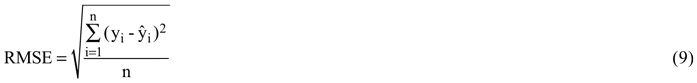

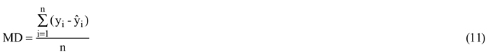

where
yi = measured value of metric y in plot i,
ŷi = predicted value of metric y in plot i,
ӯ = mean of measured values of metric y, and
n = the number of plots.
In many previous articles MD is also known as “bias”.
Because some of the models included a square root transformation of the response variable, we applied a bias correction (Lappi 1993). If
where
f(x) = function for the stem volume, biomass or dominant height and
![]() = random error,
= random error,
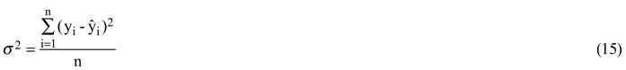
then bias correction is obtained from the equation:
where residual variance (σ2) is
2.6 Model calibration
Finally, we tested to what extent the predictions would improve if the nationwide models were calibrated locally using a small number of sample plots. The local calibration was performed using mixed-effect modelling with the same predictor metrics as used in nationwide models, and using individual inventory areas as groups. Calculations were performed by: 1) leaving inventory area “i” out; 2) fitting linear mixed-effect models with other inventory areas; 3) selecting a small number of plots from the inventory area “i”; 4) predicting the group effects of area “i” with the best linear unbiased predictor (BLUP) estimator; and 5) predicting the volume, biomass and dominant height with the created group effects, where “i” is the order number of the inventory area. The selection of local sample plots was based on quantiles of the ALS-metric havgF. The values of havgF were divided into five equal groups based on quantiles (20, 40, 60 and 80%), and four sample plots were selected from each group. Local calibration was repeated 10 000 times, and mean RMSE and MD were calculated for each inventory area. The BLUP-estimator of random effect was calculated as:
where D is the variance-covariance matrix of random effects, R is the variance-covariance matrix of residuals, Z and X both contain the same information of the ALS-metrics and y information of the field metrics of the new measured sample plots (in this case randomly selected sample plots), and β is the fixed effects of the fitted mixed-effect model (Mehtätalo and Lappi 2014). In this case we did not make assumptions for variance functions, so the residual variance-covariance matrices were created with the calculated residual variances. Residual variances were calculated in almost the same way as described before (Eq. 15), but in this case we reduced the degrees of freedom from the total number of sample plots.
3 Results
3.1 Nationwide and regional volume models
The nationwide volume model was:
where the residual variance was 2.0923. In the modelling dataset, the relative RMSE was 27.8%. The results of the t-test (Table 4) show that the nationwide model residual means differed significantly from zero in almost all of the inventory areas. The absolute values of paired-sample t-test statistics varied between 2.0 and 14.7. The null hypothesis was rejected everywhere (p < 0.05), except in the inventory area of Turku. Region-specific RMSEs of the nationwide model predictions ranged from 22.9% to 31.8% and MDs from –11.2% to 16.3%.
| Table 4. Root mean square error (RMSE), mean difference (MD) and t-test statistics of the region-specific nationwide volume model predictions. | ||||
| Inventory Area | RMSE-% | MD-% | t-value | p-value |
| Kolari | 30.1 | 15.4 | 13.7 | < 2.2×10⁻¹⁶ |
| Tornio | 28.4 | –7.4 | –6.6 | 8.5×10⁻¹¹ |
| Ranua | 31.8 | 16.3 | 14.7 | < 2.2×10⁻¹⁶ |
| Siikalatva | 25.8 | –3.6 | –3.6 | 2.9×10⁻⁴ |
| Toholampi | 24.8 | –5.5 | –5.5 | 5.4×10⁻⁸ |
| Ähtäri | 26.8 | 8.0 | 11.1 | < 2.2×10⁻¹⁶ |
| Sulkava | 30.4 | –11.2 | –9.5 | < 2.2×10⁻¹⁶ |
| Virolahti | 26.8 | –6.4 | –6.6 | 9.0×10⁻¹¹ |
| Turku | 22.9 | –1.7 | –2.0 | 5.1×10⁻² |
The regional volume models and their relative RMSE values are presented in Table 5. The MD was always zero in the modelling dataset. According to the results, the RMSEs of the regional models (ranging from Kolari’s 21.5% to Sulkava’s 26.6%) were slightly smaller than the nationwide model’s RMSE (27.8%). The most common single metric occurring in the different volume models was the mean height of first and last echoes, and its square root transformation. None of the other variables occurred frequently in the models. Fig. 2 shows the predicted values obtained from nationwide and regional volume models plotted against observed values. Scattering can be seen especially in the large values of volume, notably in the case of nationwide model.
| Table 5. Regional volume (V) models, their residual variances (σ2) and relative root mean square error (RMSE) values. The used ALS metrics (Section 2.4) were means (havgF and havgL), standard deviations (hstdF and hstdL), height quantiles (h70F, h90F, h95L and h99L) and density percentages (veg3F, veg9L and veg19L) of first (F) and last (L) echoes, and the maximum value of last echoes (hmaxL). | ||||
| Inventory area | σ² | RMSE-% | ||
| Kolari | (18) | 0.9607 | 21.5 | |
| Tornio | (19) | - | 24.0 | |
| Ranua | (20) | 1.1578 | 22.9 | |
| Siikalatva | (21) | 1.4291 | 24.4 | |
| Toholampi | (22) | 1.1254 | 24.0 | |
| Ähtäri | (23) | 1.5484 | 24.7 | |
| Sulkava | (24) | 3.2302 | 26.6 | |
| Virolahti | (25) | 2.3953 | 24.8 | |
| Turku | (26) | 1.8838 | 21.8 | |

Fig. 2. Predicted (m3 ha–1) values of nationwide and regional volume models plotted against observed values (m3 ha–1) in the modeling dataset. View larger in new window/tab.
3.2 Nationwide and regional above-ground biomass models
The nationwide biomass model was:
where the residual variance was 1.1161. In the modelling dataset, its relative RMSE was 27.2%. The results of the t-tests (Table 6) show that the nationwide model residual means differed significantly from zero in all of the inventory areas. The absolute values of paired-sample t-test statistics varied between 2.4 and 14.6. Region-specific RMSEs of the nationwide model predictions ranged from 22.2% to 32.6% and MDs from –11.9% to 16.5%.
| Table 6. Root mean square error (RMSE), mean difference (MD) and t-test statistics of the region-specific nationwide biomass model predictions. | ||||
| Inventory Area | RMSE-% | MD-% | t-value | p-value |
| Kolari | 29.7 | 11.1 | 9.3 | < 2.2×10⁻¹⁶ |
| Tornio | 29.4 | –2.9 | –2.4 | 1.7×10⁻² |
| Ranua | 32.6 | 16.5 | 14.6 | < 2.2×10⁻¹⁶ |
| Siikalatva | 25.9 | –7.1 | –7.3 | 8.9×10⁻¹³ |
| Toholampi | 25.3 | –6.8 | –6.8 | 2.8×10⁻¹¹ |
| Ähtäri | 26.0 | 8.2 | 11.6 | < 2.2×10⁻¹⁶ |
| Sulkava | 29.4 | –11.9 | –10.6 | < 2.2×10⁻¹⁶ |
| Virolahti | 26.0 | –3.9 | –4.0 | 5.9×10⁻⁵ |
| Turku | 22.2 | –2.3 | –2.7 | 6.4×10⁻³ |
The regional biomass models and their relative RMSE values are presented in Table 7. According to the results, the RMSEs of the regional models (ranging from Turku’s 20.1% to Sulkava’s 25.2%) were slightly smaller than the nationwide model’s RMSE (27.2%). In general, regional biomass RMSEs varied less than volume RMSEs. However, the predictors chosen for the regional biomass models were mostly similar to the volume models. In addition, the scatter plots between predicted and observed values was similar to the volume models (Fig. 3).
| Table 7. Regional biomass (Mt) models, their residual variances (σ2) and relative root mean square error (RMSE) values. The used ALS metrics (Section 2.4) were means (havgF, and havgL), height quantiles (h70F, h90F and h99L) and density percentages (veg3F, veg7L, veg8L and veg19L) of first (F) and last (L) echoes, standard deviation (hstdL), and the maximum value (hmaxL) of last echoes. | ||||
| Inventory area | σ² | RMSE-% | ||
| Kolari | (28) | 0.5603 | 22.0 | |
| Tornio | (29) | 0.6791 | 23.7 | |
| Ranua | (30) | 0.6465 | 23.4 | |
| Siikalatva | (31) | 0.7214 | 23.0 | |
| Toholampi | (32) | 0.5734 | 23.0 | |
| Ähtäri | (33) | 0.8074 | 23.4 | |
| Sulkava | (34) | 1.6063 | 25.2 | |
| Virolahti | (35) | 1.2081 | 23.4 | |
| Turku | (36) | 0.8717 | 20.1 | |
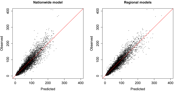
Fig. 3. Predicted (t ha–1) values of nationwide and regional biomass models plotted against observed values (t ha–1) in the modelling dataset. View larger in new window/tab.
3.3 Nationwide and regional dominant height models
The nationwide dominant height model was:
where the relative RMSE was 6.7%. The results of the t-tests (Table 8) show that the nationwide model residual means differed significantly from zero in almost all of the inventory areas. The absolute values of paired-sample t-test statistics varied between 1.1 and 28.8. The null hypothesis was rejected everywhere (p < 0.05), except in inventory areas of Kolari and Virolahti. Region-specific RMSEs of the nationwide model predictions ranged from 5.4% to 10.5% and MDs from –8.0% to 2.4%.
| Table 8. Root mean square error (RMSE), mean difference (MD) and t-test statistics of the region-specific nationwide dominant height model predictions. | ||||
| Inventory Area | RMSE-% | MD-% | t-value | p-value |
| Kolari | 7.2 | –0.4 | –1.2 | 2.2×10⁻¹ |
| Tornio | 10.5 | –8.0 | –28.8 | < 2.2×10⁻¹⁶ |
| Ranua | 7.6 | –1.7 | –5.7 | 2.3×10⁻⁸ |
| Siikalatva | 5.5 | 1.6 | 7.6 | 1.2×10⁻¹³ |
| Toholampi | 5.9 | 0.7 | 3.0 | 2.8×10⁻³ |
| Ähtäri | 6.5 | 1.4 | 7.5 | 1.4×10⁻¹³ |
| Sulkava | 6.9 | –0.8 | –2.7 | 7.7×10⁻³ |
| Virolahti | 5.4 | 0.2 | 1.1 | 2.9×10⁻¹ |
| Turku | 5.9 | 2.4 | 11.8 | < 2.2×10⁻¹⁶ |
The regional dominant height models and their relative RMSE values are presented in Table 9. The results show that the nationwide and regional dominant height models performed very well (Fig. 4). The RMSEs of the regional dominant height models vary between Siikalatva’s 5.2% and Sulkava’s 6.7%, while the nationwide RMSE was 6.7%. The most common predictors for dominant height were 95 and 99 percent first echo height quantiles.
| Table 9. Regional dominant height (HDOM) models, their residual variances (σ2) and relative root mean square error (RMSE) values. The used ALS metrics (Section 2.4) were height quantiles (h95F, h99F, h95L and h99L) of first (F) and last (L) echoes. | ||||
| Inventory Area | σ² | RMSE-% | ||
| Kolari | (38) | 0.0161 | 6.5 | |
| Tornio | (39) | - | 6.4 | |
| Ranua | (40) | - | 6.3 | |
| Siikalatva | (41) | - | 5.2 | |
| Toholampi | (42) | 0.0127 | 5.8 | |
| Ähtäri | (43) | - | 6.3 | |
| Sulkava | (44) | 0.0248 | 6.7 | |
| Virolahti | (45) | - | 5.4 | |
| Turku | (46) | - | 5.4 | |
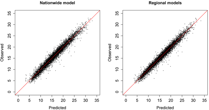
Fig. 4. Predicted (m) values of nationwide dominant height model and regional models plotted against observed values (m) in the modeling dataset. View larger in new window/tab.
3.4 Cross-validations
Table 10 presents the relative RMSE and MD values of nationwide and regional model cross-validations, and nationwide model calibration. When examining the cross-validated RMSEs and MDs of nationwide (leave-inventory-area-out) and regional (leave-plot-out) volume and biomass models, it can be noted that the nationwide models had on average smaller accuracy in northern Finland. The nationwide volume and biomass models had largest RMSE and MD in the Ranua area, where the RMSE of the nationwide volume model (32.9%) was 9.8 percentage points larger than the RMSE of the regional model (23.1%). In Ranua, the MD of the nationwide volume model was 18.2%. The lowest nationwide RMSE and MD of volume and biomass occurred in Turku, where the RMSE of the nationwide volume model (23.0%) was only 1.1 percentage points larger than with the regional model (21.9%). In Turku, the MD of the nationwide volume model was only –2.0%.
| Table 10. Relative root mean square error (RMSE) and mean difference (MD) values of cross-validated nationwide (leave-inventory-area-out) and regional (leave-plot-out) volume, biomass and dominant height models, and the calibrated nationwide models in different inventory areas. | ||||||
| RMSE-% | MD-% | |||||
| Inventory area | Nationwide | Calibrated | Regional | Nationwide | Calibrated | |
| Volume | Kolari | 31.0 | 23.9 | 21.7 | 16.8 | 3.9 |
| Tornio | 28.9 | 27.5 | 24.2 | –8.8 | –1.5 | |
| Ranua | 32.9 | 26.3 | 23.1 | 18.2 | 3.5 | |
| Siikalatva | 25.9 | 26.4 | 24.6 | –4.2 | –2.3 | |
| Toholampi | 25.0 | 24.7 | 24.3 | –6.1 | –1.9 | |
| Ähtäri | 28.0 | 26.0 | 24.8 | 10.8 | 0.8 | |
| Sulkava | 31.6 | 28.3 | 26.8 | –13.2 | –1.2 | |
| Virolahti | 27.0 | 26.7 | 25.0 | –7.5 | –0.6 | |
| Turku | 23.0 | 23.3 | 21.9 | –2.0 | –0.3 | |
| Biomass | Kolari | 30.1 | 26.3 | 22.2 | 12.1 | 2.9 |
| Tornio | 29.6 | 29.0 | 23.9 | –3.5 | –0.3 | |
| Ranua | 33.8 | 27.7 | 23.6 | 18.7 | 4.3 | |
| Siikalatva | 26.1 | 25.5 | 23.2 | –8.0 | –2.8 | |
| Toholampi | 25.6 | 24.4 | 23.2 | –7.6 | –1.9 | |
| Ähtäri | 27.3 | 24.1 | 23.5 | 10.8 | 1.5 | |
| Sulkava | 30.3 | 27.0 | 25.4 | –13.8 | –1.7 | |
| Virolahti | 26.1 | 25.7 | 23.6 | –4.4 | –0.1 | |
| Turku | 22.3 | 21.9 | 20.2 | –2.6 | –0.3 | |
| Dominant height | Kolari | 7.2 | 7.4 | 6.5 | –0.4 | 0.0 |
| Tornio | 11.4 | 8.2 | 6.4 | –9.1 | –4.6 | |
| Ranua | 7.7 | 7.6 | 6.3 | –2.0 | –0.3 | |
| Siikalatva | 5.5 | 5.3 | 5.2 | 1.7 | 0.4 | |
| Toholampi | 6.0 | 5.9 | 5.8 | 0.8 | 0.1 | |
| Ähtäri | 6.6 | 6.4 | 6.3 | 1.7 | 0.3 | |
| Sulkava | 6.9 | 6.9 | 6.7 | –0.9 | –0.2 | |
| Virolahti | 5.4 | 5.5 | 5.4 | 0.2 | 0.1 | |
| Turku | 6.1 | 5.6 | 5.4 | 2.8 | 0.9 | |
However, with the exception of one region, the results of cross-validation showed that nationwide dominant height models performed well across the whole country. The one exception was Tornio where the nationwide model MD was –9.1% and the corresponding RMSE (11.4%), 5.0 percentage points larger than the RMSE of the regional model (6.4%). Otherwise, the largest dominant height nationwide RMSE was seen in Ranua (7.7%), which differed only 1.4 percentage points from the regional model RMSE (6.3%). The lowest RMSE of the nationwide dominant height model (5.4%) was in Virolahti, where there was almost no difference to the regional model (5.4%). Correspondingly, the largest MD was in the Turku region with 2.8%, and closest to zero in Virolahti with 0.2%. Fig. 5 shows the geographical distributions of the nationwide MDs, with information of the different sensor models and units that were used.
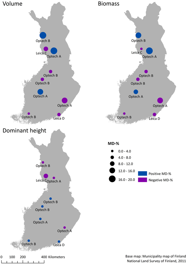
Fig. 5. Map of the mean difference (MD) values of nationwide volume, biomass and dominant height models with information of different sensor models (Optech/Leica) and sensor units (A–D).
3.5 Effects of the ALS devices on mean difference in nationwide models
As mentioned above, we used two different sensor models and four different sensor units in this study. Thus, we examined how the individual sensor model or unit affected the evidence of MD in nationwide predictions. According to a subjective evaluation between Tables 3 and 10, it can be noted that MDs of volume and biomass models were on average larger when the inventory area was scanned with Optech, rather than with Leica scanners. Differences can be likewise noted between the sensor units. For example, on average the Optech unit B provided smaller MD values than unit A in the case of volume and biomass. There was also some evidence that the PRF and scan angle may possibly affect the MD. When the PRF was 50 000 hz and the scan angle was 15 degrees, then predictions in the nationwide biomass and volume models showed a larger MD compared to parameters of 70 000 hz and 20 degrees. We also tried to fit the nationwide volume model only with metrics in first echo category (F), because the last echoes (L) are usually more affected by sensor variability (Næsset 2005). However, the results of the leave-inventory-area-out cross validation showed that nationwide volume models with only first echo metrics have on average a 0.2 percentage points larger RMSE and exactly the same MD than the original nationwide model (Eq. 17).
3.6 Local calibration
Local calibration improved the predictions in all of the areas. Especially, the MDs decreased everywhere. On the scale of the whole country, the MD of the nationwide volume model decreased on average 8.0 percentage points (11.6 percentage points in the north and 6.1 percentage points in the south), and the MD of the nationwide biomass model decreased 7.3 percentage points (north 8.9, south 6.5). The RMSEs of the calibrated nationwide model approached regional values, but less so than was seen in regard to MDs. With the exceptions of Siikalatva and Turku, the RMSE of the nationwide volume model decreased on average 3.0 percentage points (north 5.0, south 1.5). However, in Siikalatva and Turku, the uncalibrated nationwide RMSE was very close to the regional RMSE. In the case of nationwide biomass model, the RMSE decreased in all of the inventory areas with an average of 2.2 percentage points (north 3.5, south 1.5). The RMSEs and MDs of nationwide volume and biomass models were most reduced in the northern part of Finland. The difference in calibrated nationwide volume model RMSEs to regional RMSEs was on average 1.9 percentage points (north 2.9, south 1.3). The corresponding difference to the biomass models was 2.5 percentage points (north 4.4, south 1.6). No substantial benefits were gained by calibration of the nationwide dominant height model. Calibrated nationwide dominant height model RMSEs approached the regional models, with the exceptions of Kolari and Virolahti, and the MDs approached zero in all of the study areas. However, the RMSE and MD of dominant height was seen to stay relatively larger in Tornio with 8.2% and –4.6%.
The RMSE and MD distributions from the 10 000 calibrations are presented in Fig. 6–11. The volume RMSE distributions were not uniform. In almost all of the inventory areas, the RMSE means of the calibrated volume model fell on the right side of the highest distribution bar. In the case of biomass, the means usually coincided with the peak of the distribution. However, the MDs of volume and biomass predictions were very uniformly distributed, although the distributions were relatively wide. The standard deviations of MDs were much larger than the standard deviations of RMSEs. The shapes of the dominant height RMSE and MD distributions were similar to the volume and biomass distributions, but their standard deviations were smaller.
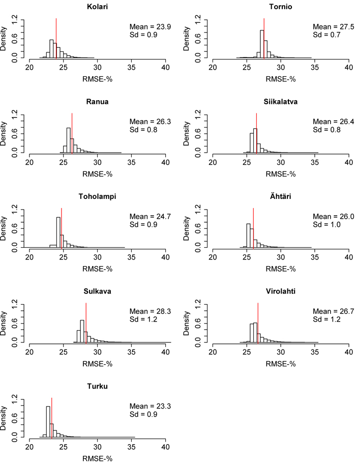
Fig. 6. Root mean square error (RMSE) distributions of the 10 000 times calibrated nationwide volume model in each inventory area. The red line represents the mean of the distribution. Sd = Standard deviation. View larger in new window/tab.
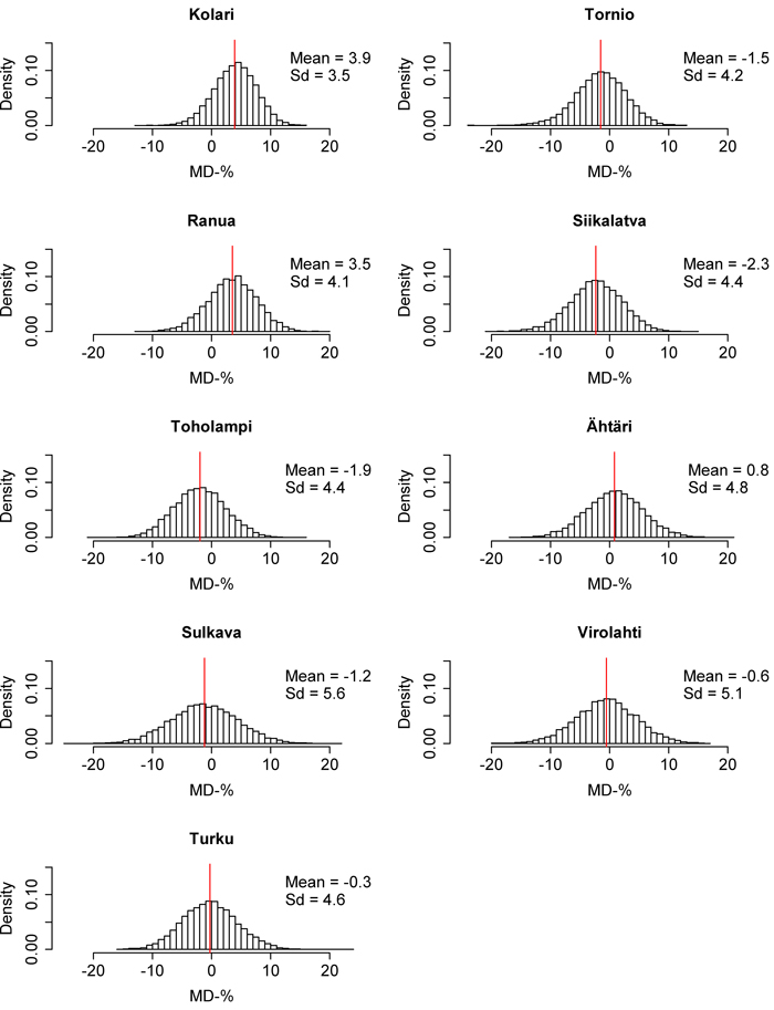
Fig. 7. Mean difference (MD) distributions of the 10 000 times calibrated nationwide volume model in each inventory area. The red line represents the mean of the distribution. Sd = Standard deviation. View larger in new window/tab
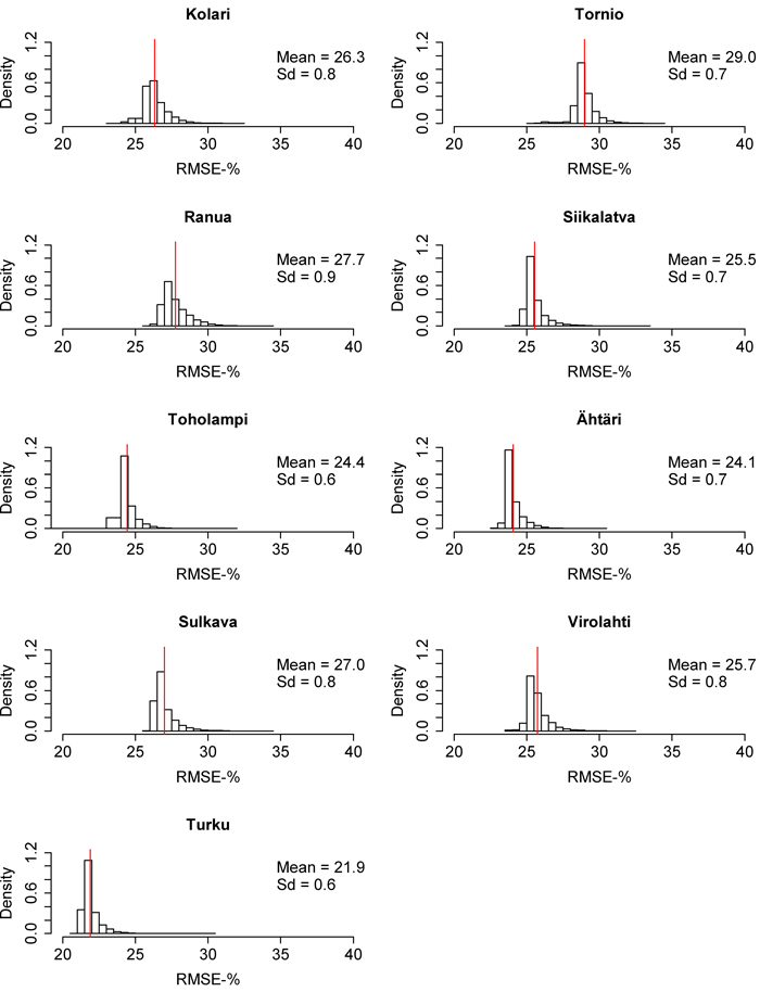
Fig. 8. Root mean square error (RMSE) distributions of the 10 000 times calibrated nationwide biomass model in each inventory area. The red line represents the mean of the distribution. Sd = Standard deviation. View larger in new window/tab
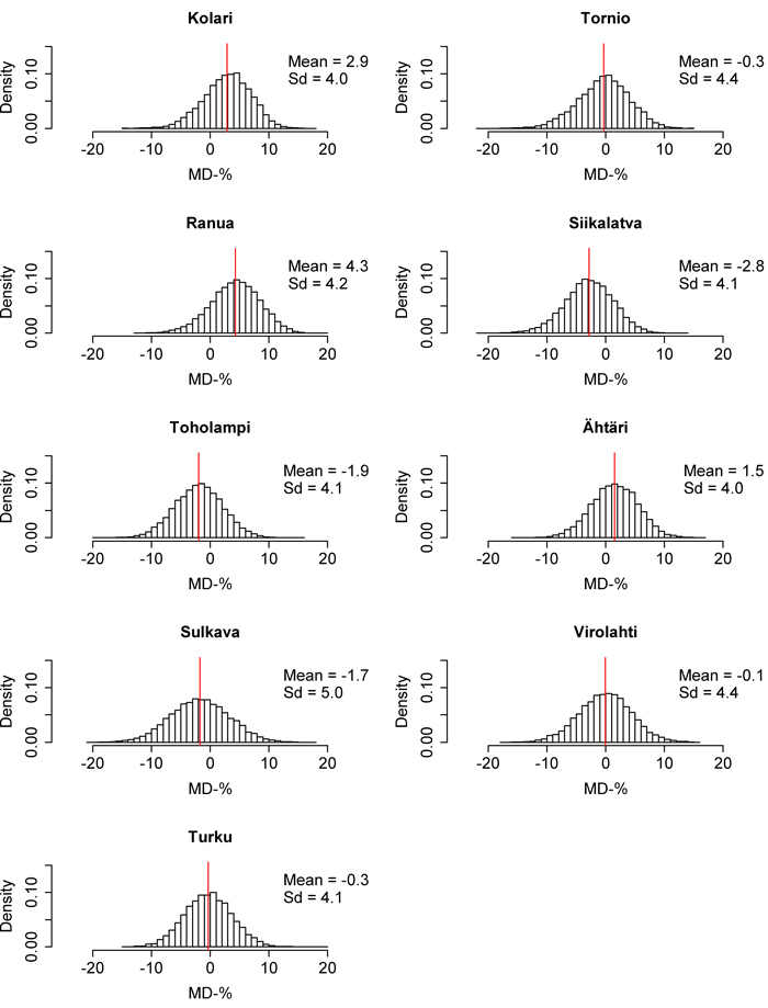
Fig. 9. Mean difference (MD) distributions of the 10 000 times calibrated nationwide biomass model in each inventory area. The red line represents the mean of the distribution. Sd = Standard deviation. View larger in new window/tab
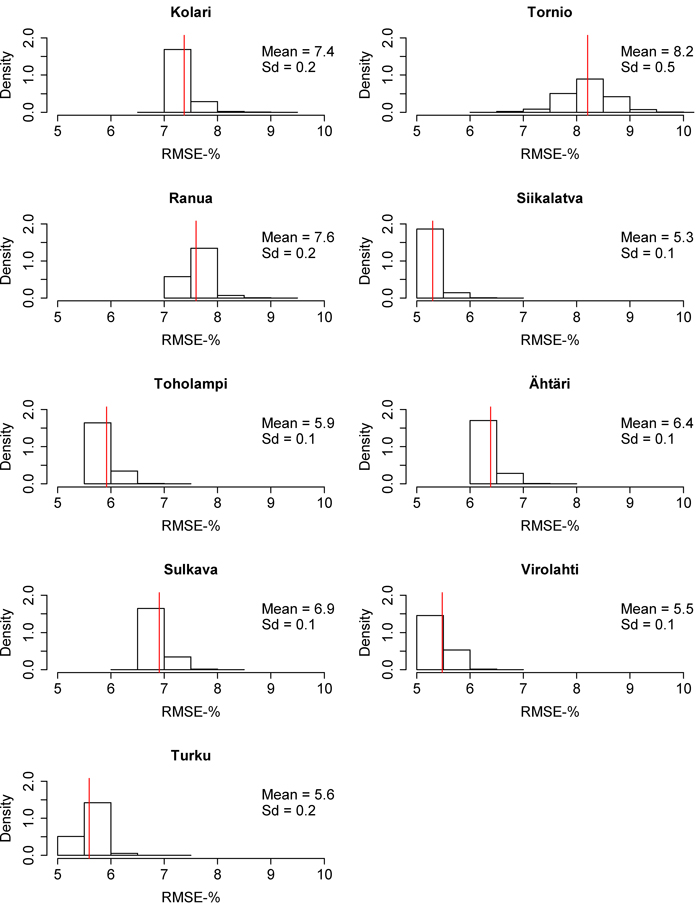
Fig. 10. Root mean square error (RMSE) distributions of the 10 000 times calibrated nationwide dominant height model in each inventory area. The red line represents the mean of the distribution. Sd = Standard deviation. View larger in new window/tab
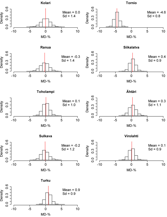
Fig. 11. Mean difference (MD) distributions of the 10 000 times calibrated nationwide dominant height model in each inventory area. The red line represents the mean of the distribution. Sd = Standard deviation. View larger in new window/tab
4 Discussion
Although forest structures differ among different parts of Finland, it is still possible to obtain rather good predictions with nationwide volume and biomass models. In general, a risk of MD has to be accepted if the nationwide volume and biomass models are applied in practice. For example, in the cross-validation of the nationwide volume model, the absolute averages of MDs were clearly different in southern (7.3%) and northern (14.6%) Finland. For biomass, the corresponding values were 7.9% and 11.4%. The MD differences between the nationwide volume and biomass models in the north were caused by the Tornio area, where the predictions of the biomass model had smaller MD than the predictions of the volume model. Location of inventory area seems to affect the predictions of the nationwide models. The residual means of the nationwide model’s regional predictions differed significantly from zero in most of the inventory areas (Tables 4, 6 and 8). Prediction accuracy is probably affected by both the different forest structures and the use of different ALS devices. Therefore, predictions could probably be improved if models were created separately for different ALS devices (as also reported by Næsset 2009). We noted that there were clear differences in regional MDs between Optech scanners. There was also a difference between Leica scanners, but because there were only two of these sensor units, no major conclusions can be drawn. The results of nationwide volume models are in line with the findings of Suvanto and Maltamo (2010). In their study, the RMSE of a general volume model (with merged dataset using all sample plots) was about 25%, and RMSE of the local model (with separate variable selection) was about 20%, which are comparable to our results (Table 4). According to Suvanto and Maltamo (2010), their results were also influenced by two different ALS devices.
Overall, the nationwide dominant height model performed well across the whole country, with the exception of the inventory area of Tornio. In the other areas, the absolute average of MDs was only 1.3%. Good performance with dominant height models was predictable because the ALS data directly describes the height of the tallest trees. The offset in Tornio is interesting, but the difference between nationwide and regional predictions could be related to crown shape. In Tornio, the 99th quantile of the first echoes was applied as the predictor in the local height model, while the nationwide model was based on the 95th quantile. If the crown shape in Tornio was different from the rest of the country, then the 99th quantile may explain the height variations of the tallest trees more accurately than the 95th quantile. Moreover, the used Leica scanner could also have an effect on the dominant height predictions of Tornio, but a clear comparison between the sensor models and units cannot be made because of small MDs which were noted in the other eight areas.
In Finnish ALS-based inventory projects, it is typical to predict species-specific stand attributes by nearest neighbor imputation using a combination of ALS data and aerial photographs (Packalén and Maltamo 2007). According to Packalén and Maltamo (2007), the RMSE of the sum of the species-specific volume predictions was 20.5% in the Matalansalo study area, which is 2.5–12.4 (mean 7.6) percentage points lower than the RMSEs of our nationwide model. This species-specific RMSE of volume is also, 1.2–6.3 (mean 3.5) percentage points lower than the RMSEs of our regional models. However, small differences in RMSE between different inventory areas are very common, and the size of the area featured in the study of Packalén and Maltamo (2007) was limited. Also, an advantage in using the nearest neighbor imputation approach is to enable species-specific predictions, which are not possible to obtain using our nationwide volume model. However, RMSE clearly decreases when models are applied on a stand level. According to Packalén and Maltamo (2007), the RMSE of volume predictions was about 10.4% when the species-specific predictions were generalized to a stand level. Correspondingly, similar results can be obtained when the stand volume is predicted using combined data from two districts (Næsset 2007). According to Næsset (2007), the RMSEs of volume and dominant height were around 10.6% to 14.0% and 3.4% to 3.7% depending on the forest type. The corresponding MDs were 1.5% to 6.7%, and –1.7% to 0.7%, respectively. It remains an open question, how RMSE and MD could change if nationwide models are used to predict stand level attributes, but most likely they would show a clear decrease. In a national level ALS inventory based on Swedish NFI plots, the stand level RMSEs of stem volume ranged from 17.2% to 23.3% (Nilsson et al. 2015). We expect that the stand level RMSE values of our nationwide model could be equally good.
Although the comparison between the plot and stand level is not straightforward, we can say that our nationwide models work fairly well compared to traditional stand level inventory in Finland. In Finland, the traditional stand level inventory is based on visual stand delineation, randomly placed angle count sampling plots, and species-specific basal area median tree measurements (Haara and Korhonen 2004). According to the results of Haara and Korhonen (2004), it is possible to obtain on average about a 25% RMSE for volume with the traditional stand level inventory method, which is about 1–8 (mean 4) percentage points lower than the RMSEs of our nationwide volume model at the plot level. In the inventory area of Toholampi, the plot level accuracy of our model was equal to the traditional stand level field inventory (such as that featured in Haara and Korhonen 2004), and in Turku our model was even more accurate. Probably, if we utilized nationwide models to a stand level, then there would be a possibility of obtaining even smaller RMSEs in every region than using traditional stand level inventory methods. The bias in traditional stand level inventory was only 1.6% (Haara and Korhonen 2004), which is considerably smaller than the MDs seen in our nationwide volume model (–13.2% to 18.2%). However, with only a couple of days of field measurements and model calibration, it is possible to reduce the MD of nationwide model (–2.3% to 3.9%).
As noted above, local calibration improves the predictions of nationwide volume and biomass models, and in this study, after calibration, the absolute averages of volume model MDs were only 1.2% in the south and 3.0% in the north. Corresponding values for the nationwide biomass model were 1.4% and 2.5% respectively. Calibration improves volume and biomass predictions by fixing the estimated relationships between ALS and field data, in order to describe the structural properties of forests in the new target area more accurately (Næsset et al. 2005). In the case of dominant height, calibration did not bring about substantial benefits, because the uncalibrated nationwide model already performed well. However, it should be remembered that the results of local calibration may vary depending on the chosen sample plots. Because of this, historical data from previous inventories and ALS-derived metrics of the area are important in sample plot placement (Hawbaker et al. 2009).
RMSE distributions showed that the mean RMSE values of 10 000 calibrated nationwide models did not accurately represent the real situation of nationwide model calibration. Especially in the case of volume, the RMSE distributions were not uniform and some very large values tended to increase the overall averages. For this reason, our mean RMSEs alone may not give a realistic picture of the calibration, if the sampling design is well-planned. When we examined the RMSE values of calibration in more detail, we found that with some sample plot combinations it was possible to construct a calibration that provided even more accurate predictions than those of regional models. Therefore, the issue of sampling for local calibration still requires further research.
5 Conclusions
The accuracy of general volume (and biomass) model predictions (RMSE 22% to 34%) was comparable to relascope-based field inventory by compartments. However, the mean of the predicted values will usually differ from the real mean, especially if there are variations in site quality within the application area. Differences in forest structure and the use of different ALS devices influence the accuracy of nationwide models, but region-specific calibration can improve the model performance considerably. In most of the regions the nationwide model’s dominant height predictions were as good as regional predictions.
Acknowledgements
The authors thank the Finnish Forestry Center, Blom Kartta Oy, TerraTec Oy and the National Land Survey of Finland for their co-operation during this work. Lauri Korhonen was also supported by the Academy of Finland.
References
Axelsson P. (2000). DEM generation from laser scanner data using adaptive TIN models. International Archives of Photogrammetry and Remote Sensing 33(B4): 110–117.
Blom Kartta Oy (2012). Maastomittauksen työohje. [Working instructions of field measurement]. 4 p.
Breidenbach J., Kublin E., McGaughey R.J., Andersen H.-E., Reutebuch S.E. (2008). Mixed effect models for estimating stand volume by means of small footprint airborne laser scanner data. The Photogrammetric Journal of Finland 21(1): 4–15.
Delang C.O., Li W.M. (2013). Forest structure. In: Ecological succession on fallowed shifting cultivation fields. A review of the literature. Springer. p. 9–37. http://dx.doi.org/10.1007/978-94-007-5821-6_2.
Haara A., Korhonen K.T. (2004). Kuviottaisen arvioinnin luotettavuus. [Accuracy of stand level mensuration]. Metsätieteen aikakauskirja 4/2004: 489–508.
Hawbaker T.J., Keuler N.S., Lesak A.A., Gobakken T., Contrucci K., Radeloff V.C. (2009). Improved estimates of forest vegetation structure and biomass with a LiDAR-optimized sampling design. Journal of Geophysical Research 114(G2). 11 p. http://dx.doi.org/10.1029/2008JG000870.
Hopkinson C. (2007). The influence of flying altitude, beam divergence, and pulse repetition frequency on laser pulse return intensity and canopy frequency distribution. Canadian Journal of Remote Sensing 33(4): 311–324. http://dx.doi.org/10.5589/m07-029.
Hyndman R.J., Fan Y. (1996). Sample quantiles in statistical packages. The American Statistician 50(4): 361 – 365.
Kangas A., Päivinen R., Holopainen M., Maltamo M. (2011). Silva Carelica 40. Metsänmittaus ja kartoitus. [Forest mensuration and mapping]. University of Eastern Finland, School of Forest Sciences. 210 p.
Laasasenaho J. (1982). Taper curve and volume functions for pine, spruce and birch. Communicationes Instituti Forestalis Fenniae 108. 74 p.
Lappi L. (1993). Metsäbiometrian menetelmiä. [Methods of forest biometrics]. University of Joensuu, Faculty of Forest Sciences, Silva Carelica 24. 182 p.
Maltamo M., Packalen P. (2014). Species-specific management inventory in Finland. In: Maltamo M., Næsset E., Vauhkonen J. (eds.). Forestry applications of airborne laser scanning - concepts and case studies. Managing Forest Ecosystems 27. Springer. p. 241–252. http://dx.doi.org/10.1007/978-94-017-8663-8_12.
Mehtätalo L., Lappi J. (2014). Forest biometrics with examples in R. Textbook manuscript in preparation for Chapman & Hall. 156 p.
Metla [Finnish Forest Research Institute], Suomen Metsäkeskus [Finnish Forestry Centre] (2013). VMI-SMKI Maastotyöohje. [The field measurement guide]. 23 p.
Metsäntutkimuslaitos [Finnish Forest Research Institute] (2014). Metsätilastollinen vuosikirja. [Finnish Statistical Yearbook of Forestry]. http://www.metla.fi/metinfo/tilasto/julkaisut/vsk/2014/index.html. [Cited 23 Nov 2015].
Næsset E. (2002). Predicting forest stand characteristics with airborne scanning laser using a practical two-stage procedure and field data. Remote Sensing of Environment 80(1): 88–99. http://dx.doi.org/10.1016/S0034-4257(01)00290-5.
Næsset E. (2004) Effects of different flying altitudes on biophysical stand properties estimated from canopy height and density measured with a small footprint airborne scanning laser. Remote Sensing of Environment 91(2): 243–255. http://dx.doi.org/10.1016/j.rse.2004.03.009.
Næsset E. (2005). Assessing sensor effects and effects of leaf-off and leaf-on canopy conditions on biophysical stand properties derived from small-footprint airborne laser data. Remote Sensing of Environment 98(2–3): 356–370. http://dx.doi.org/10.1016/j.rse.2005.07.012.
Næsset E. (2007). Airborne laser scanning as a method in operational forest inventory: status of accuracy assessment accomplished in Scandinavia. Scandinavian Journal of Forest Research 22(5): 433–442. http://dx.doi.org/10.1080/02827580701672147.
Næsset E. (2009). Effects of different sensors, flying altitudes, and pulse repetition frequencies on forest canopy metrics and biophysical stand properties derived from small-footprint airborne laser data. Remote Sensing of Environment 113(1): 148–159. http://dx.doi.org/10.1016/j.rse.2008.09.001.
Næsset E. (2014). Area-based inventory in Norway – from innovation to an operational reality. In: Maltamo M., Næsset E., Vauhkonen J. (eds.). Forestry applications of airborne laser scanning - concepts and case studies. Managing Forest Ecosystems 27. Springer. p. 215–240. http://dx.doi.org/10.1007/978-94-017-8663-8_11.
Næsset E., Gobakken T. (2008). Estimation of above- and below- gound biomass across regions of the boreal forest zone using airborne laser. Remote Sensing of Environment 112(6): 3079–3090. http://dx.doi.org/10.1016/j.rse.2008.03.004.
Næsset E., Bollandsås O.M., Gobakken T. (2005). Comparing regression methods in estimation of biophysical properties of forest stands from two different inventories using laser scanner data. Remote Sensing of Environment 94(4): 541–553. http://dx.doi.org/10.1016/j.rse.2004.11.010.
Nilsson M., Nordkvist K., Jonzén J., Lindgren N., Axensten P., Wallerman J., Egberth M., Larsson S., Nilsson L., Eriksson J., Olsson H. (2015). A nationwide forest attribute map of Sweden derived using airborne laser scanning data and field data from the national forest inventory. Proceedings of SilviLaser, 14th conference on Lidar Applications for Assessing and Managing Forest Ecosystems, September 28–30, La Grande Motte, France. p. 211–213.
Packalén P., Maltamo M. (2007). The k-MSN method for the prediction of species-specific stand attributes using airborne laser scanning and aerial photographs. Remote Sensing of Environment 109(3): 328–341. http://dx.doi.org/10.1016/j.rse.2007.01.005.
Ratilainen A. (2011). User guide, TTFIELD 2.0 etc. TerraTec Oy, Helsinki. 4 p.
Repola J. (2008). Biomass equations for birch in Finland. Silva Fennica 42(4): 605–624. http://dx.doi.org/10.14214/sf.236.
Repola J. (2009). Biomass equations for Scots pine and Norway spruce in Finland. Silva Fennica 43(4): 625–647. http://dx.doi.org/10.14214/sf.184.
Suomen Metsäkeskus [Finnish Forestry Centre] (2014). Kaukokartoitusperusteisen metsien inventoinnin koealojen maastotyöohje, versio 1.4. [The remote sensing based forest inventory field guide for plot measurements, version 1.4]. 27 p.
Suvanto A., Maltamo M. (2010). Using mixed estimation for combining airborne laser scanning data in two different forest areas. Silva Fennica 44(1): 91–107. http://dx.doi.org/10.14214/sf.164.
Vauhkonen J., Maltamo M., McRoberts R.E., Næsset E. (2014). Introduction to forest applications of airborne laser scanning. In: Maltamo M., Næsset E., Vauhkonen J. (eds.). Forestry applications of airborne laser scanning - concepts and case studies. Managing Forest Ecosystems 27. Springer. p. 1–16. http://dx.doi.org/10.1007/978-94-017-8663-8_1.
Villikka M., Packalén P., Maltamo M. (2012). The suitability of leaf-off airborne laser scanning data in an area-based forest inventory of coniferous and deciduous trees. Silva Fennica 46(1): 99–110. http://dx.doi.org/10.14214/sf.68.
Total of 32 references.
