Jonas Bohlin  ,
Inka Bohlin,
Jonas Jonzén,
Mats Nilsson
,
Inka Bohlin,
Jonas Jonzén,
Mats Nilsson
Mapping forest attributes using data from stereophotogrammetry of aerial images and field data from the national forest inventory
Bohlin J., Bohlin I., Jonzén J., Nilsson M. (2017). Mapping forest attributes using data from stereophotogrammetry of aerial images and field data from the national forest inventory. Silva Fennica vol. 51 no. 2 article id 2021. https://doi.org/10.14214/sf.2021
Highlights
- Image based forest attribute map generated using NFI plots show similar accuracy as currently used LiDAR based forest attribute map
- Also similar accuracies were found for different forest types
- Aerial images from leaf-off season is not recommended.
Abstract
Exploring the possibility to produce nation-wide forest attribute maps using stereophotogrammetry of aerial images, the national terrain model and data from the National Forest Inventory (NFI). The study areas are four image acquisition blocks in mid- and south Sweden. Regression models were developed and applied to 12.5 m × 12.5 m raster cells for each block and validation was done with an independent dataset of forest stands. Model performance was compared for eight different forest types separately and the accuracies between forest types clearly differs for both image- and LiDAR methods, but between methods the difference in accuracy is small at plot level. At stand level, the root mean square error in percent of the mean (RMSE%) were ranging: from 7.7% to 10.5% for mean height; from 12.0% to 17.8% for mean diameter; from 21.8% to 22.8% for stem volume; and from 17.7% to 21.1% for basal area. This study clearly shows that aerial images from the national image program together with field sample plots from the NFI can be used for large area forest attribute mapping.
Keywords
airborne laser scanning;
National Forest Inventory;
photogrammetry;
aerial images;
forest attribute estimation;
image matching;
large area
-
Bohlin,
Department of Forest Resource Management, Swedish University of Agricultural Sciences, S-901 35 Umeå, Sweden
 http://orcid.org/0000-0002-3318-5967
E-mail
jonas.bohlin@slu.se
http://orcid.org/0000-0002-3318-5967
E-mail
jonas.bohlin@slu.se
-
Bohlin,
Department of Forest Resource Management, Swedish University of Agricultural Sciences, S-901 35 Umeå, Sweden
http://orcid.org/0000-0003-1224-6684
E-mail
inka.bohlin@slu.se
- Jonzén, Department of Forest Resource Management, Swedish University of Agricultural Sciences, S-901 35 Umeå, Sweden E-mail jonas.jonzen@slu.se
-
Nilsson,
Department of Forest Resource Management, Swedish University of Agricultural Sciences, S-901 35 Umeå, Sweden
http://orcid.org/0000-0001-7394-6305
E-mail
mats.nilsson@slu.se
Received 19 January 2017 Accepted 19 April 2017 Published 21 April 2017
Views 131433
Available at https://doi.org/10.14214/sf.2021 | Download PDF

1 Introduction
Mapping of forest attributes using light detection and ranging (LiDAR) has recently changed how forest companies acquire forest information. Airborne Laser Scanning (ALS) based forest inventories are now common practice in many countries (White et al. 2013; Vauhkonen et al. 2014). For large forest holders or groups of small forest holders with regionally concentrated forest holdings e.g., forest companies, dedicated ALS campaigns together with simultaneous field inventories of training plots is feasible, but is not cost-efficient for small forest holdings.
Small-area forest stakeholders, e.g., private forest owners, as well as governmental organisations have an interest in a production of nation-wide ALS based forest attribute maps. Many countries, e.g. Denmark, Finland, Netherland, Switzerland and Sweden, are doing or have done national ALS surveys. In Denmark, the national ALS datasets and National Forest Inventory (NFI) data has been used to estimate forest resources, reporting RMSEs of 42% for basal area and 46% for volume at plot level (Nord-Larsen and Schumacher 2012). In Austria, low point density ALS acquired for elevation mapping together with NFI data collected under operational conditions were used for wide-area stem volume estimation, resulting in standard deviation of 31.5% at plot level (Hollaus et al. 2009). In Finland, National Forest Inventory (NFI) data has been added to ALS data and dedicated field measurements for improving regional ALS based inventories done by State Forest Centres (Tuominen et al. 2014). The study showed that the accuracies of species-specific volume estimates improved by adding the NFI data, but the accuracies of total volume, stand mean height and diameter did not improve.
In Sweden, the Forest Agency (Skogsstyrelsen) is now mapping forest attributes for the whole of Sweden using ALS data captured for the ongoing production of a new national digital elevation model together with field sample plot data from the NFI (Nilsson et al. 2016). The national collection of ALS data started in 2009 and had by the end of 2016 covered more the 97% of the productive forest land area of Sweden. The national forest attribute map with estimates of stem volume, tree height, diameter, basal area, and tree biomass has been made available online for free at the Forest Agency’s web site. This has generated wide use of the dataset by different stakeholders. However, this data are rapidly aging – every year 3.5% of the forest land is changed due to forest treatments like; clear-cutting, thinning, cleaning or final felling of seedling trees (Nilsson et al. 2015). Therefore, organisations providing information to the private forest owners (e.g., the Forestry Agency and forest owner associations) are now interested in possible future updates of the national forest attribute map.
Aerial images have emerged as one possible source of data that can be used to derive three-dimensional (3D) data similar to those generated by ALS (Baltsavias 1999; Leberl et al. 2010). 3D data from aerial images describes only the upper part of the canopy surface, whereas LiDAR penetrates the canopy and also measures the vertical canopy structure and the ground. Many studies have shown that 3D data from aerial images together with a high resolution elevation model can be used to map forest attributes with accuracies similar to those obtained in ALS based forest inventories (St-Onge et al. 2008; Bohlin et al. 2012; White et al. 2013; Gobakken et al. 2015). In Switzerland, the NFI uses 3D data from aerial images (Ginzler and Hobi 2015) and NFI sample plots and a method that utilizes the NFI criteria of minimum tree height, crown coverage, width, and land use to produce a forest cover map with high accuracy, 97%, and with national cover and regular updating (Waser et al. 2015). The National Land Survey in Sweden (Lantmäteriet) annually acquires aerial images of about one third of the country, with a ground sampling distance (GSD) of 0.25 m or 0.5 m and with a forward overlap of 60% and a side overlap of 30% (base to height ratio of 0.34), ensuring that each point on the ground is represented in at least one stereo model. This is a highly interesting source of 3D data for large-area mapping of forest attributes in Sweden.
When using aerial images over large areas together with NFI sample plots to map forest attributes, some factors that affect the estimation accuracy of the mapped attributes must be addressed. The aerial image acquisitions are normally planed in large image blocks which are photographed over the time of a few days. However, difference in time over the day generates variation of the lighting conditions in the images, e.g., shadows may move between flying two strips covering the same area (Honkavaara et al. 2012) . Also due to changing weather, parts of the block may be flown later in the season. It is important to have enough field samples to describe the variation in the attributes being mapped. The Swedish NFI uses a systematic sampling design, commonly used to cover geographical variation (Maltamo et al. 2011). Nevertheless, using too old plots data or data from plots geographically too far away from the area being modelled may reduce the estimation accuracy.
In this study, the aim is to evaluate the accuracy of forest attribute mapping using 3D data from standard aerial images from the national image acquisition program in Sweden, in combination with sample plot data from the NFI. Basal area weighted mean height (Hbw), basal area weighted mean diameter (Dbw), stem volume (Vol), and basal area (BA) are mapped using the area-based approach (Næsset 2002; Næsset 2014). Model performance is reported at plot level and for different forest types and compared with model performance from ALS based models. Estimation accuracy is evaluated at stand level using independent validation datasets. In addition, models for one sub-area are applied to other sub-areas to evaluate the effect of phenological variations (leaf-on/off) and model robustness for different geographical variations, like forest structure and composition.
2 Materials and methods
2.1 Study area and training data
The study was conducted in four image acquisition blocks (sub-areas) with the size of about 10 000 km2 in southern (E2) and central (N2, Q2, R2) Sweden (Fig. 1). In each sub-area, forests consist of all kind of developing stages and are mainly dominated by conifers; Scots Pine (Pinus sylvestris L.) and Norway spruce (Picea abies L.), but deciduous trees, especially Birch (Betula spp.), occurs as minority. Forests are largely well-managed owned by both forest companies and private land owners.
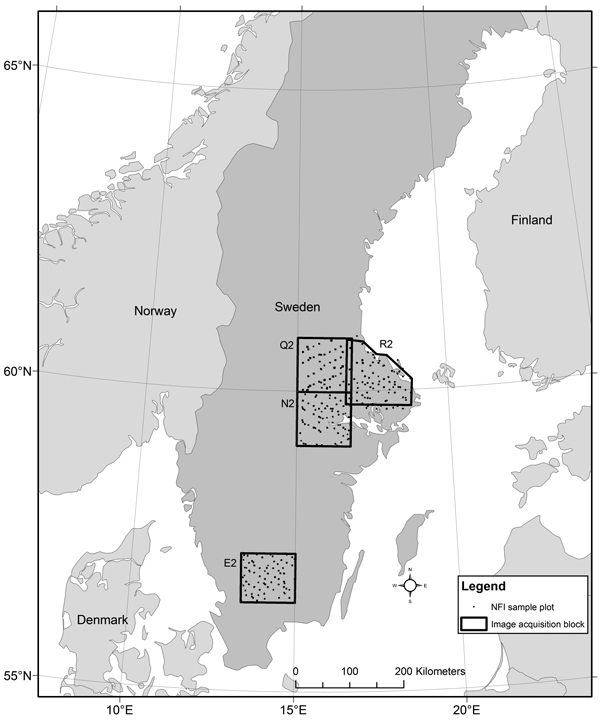
Fig. 1. The location of the four sub-areas (E2, N2, Q2 and R2) on a background map of the Nordic countries (©ESRI).
In the Swedish NFI approximately 9500 sample plots are field surveyed annually. Of these, 60% are permanent plots with a plot radius of 10 m that are revisited every five years while the remaining 40% are temporary plots with a 7 m radius. The NFI plots are positioned with GPS receivers giving a positional accuracy of about 5 m. These plots are organized into square or rectangular clusters consisting of 4, 6 or 8 plots and with a distance between plots ranging from 300 to 600 m. For this study NFI plots were selected from the same year or 1–2 years before aerial image acquisition to provide a sufficient sample of training data (Table 1). For N2 and Q2 NFI data from 2014 and for R2 NFI data from 2015 were not yet available in time of modelling. NFI plots covered forests from different developing stages and tree species composition (Table 2). In this study both permanent and temporary plots in productive forest land with Hbw over 3 meters were used. For these plots all trees was calipered. Plots recorded as divided (i.e., plots located on the boundary between two or more stands) in the field by the NFI was not used. Plots with seed trees and plots where the height of vegetation was clearly different compared to canopy height from the remotely sensed data (caused by, e.g., clear cuts made in the time period between the field inventory and the remote sensed data collections) were visually inspected and excluded, removing 10–15% of the plots depending on sub-area. This was done separately for the image and LiDAR data sets due to their time difference.
| Table 1. Data collection year for sub-areas E2, N2, Q2 and R2. | ||||
| E2 | N2 | Q2 | R2 | |
| NFI plots | 2012–2013 | 2012–2013 | 2012–2013 | 2013–2014 |
| Company stands | 2014 | - | 2015 | 2015 |
| Biotope stands | 2012–2014 | - | 2012–2015 | 2012–2015 |
| Aerial images | leaf-on 2013 | leaf-on 2014 | leaf-off 2014 | leaf-on 2015 |
| LiDAR data | 2010–2012 | 2010–2012 | 2009–2011 | 2009–2012 |
| Table 2. Summary of basal area weighted mean height (Hbw), basal area weighted mean diameter (Dbw), stem volume (Vol), and basal area (BA) of the training data for sub-areas E2, N2, Q2 and R2. Species proportion is proportion of basal area. | ||||
| Characteristic | Minimum | Maximum | Mean | Standard deviation |
| E2, n = 216 plots | ||||
| Hbw, m | 3.0 | 28.2 | 14.3 | 6.2 |
| Dbw, cm | 1.3 | 43.4 | 18.2 | 9.4 |
| BA, m2 ha–1 | 0.7 | 61.3 | 21.3 | 12.4 |
| Vol, m3 ha–1 | 2.4 | 669.1 | 168.6 | 131.1 |
| Pine proportion (%) | 0 | 100 | 21 | 31 |
| Spruce proportion (%) | 0 | 100 | 49 | 36 |
| Deciduous proportion (%) | 0 | 100 | 30 | 35 |
| N2, n = 167 plots | ||||
| Hbw, m | 3.0 | 30.8 | 15.9 | 6.1 |
| Dbw, cm | 3.5 | 42.8 | 21.0 | 9.1 |
| BA, m2 ha–1 | 1.0 | 50.8 | 22.3 | 10.4 |
| Vol, m3 ha–1 | 2.7 | 627.1 | 181.4 | 117.7 |
| Pine proportion (%) | 0 | 100 | 34 | 36 |
| Spruce proportion (%) | 0 | 100 | 38 | 32 |
| Deciduous proportion (%) | 0 | 100 | 28 | 32 |
| Q2, n = 223 plots | ||||
| Hbw, m | 3.1 | 28.4 | 15.0 | 5.9 |
| Dbw, cm | 2.8 | 41.2 | 19.0 | 8.4 |
| BA, m2 ha–1 | 2.7 | 50.5 | 22.0 | 9.9 |
| Vol, m3 ha–1 | 6.6 | 547.9 | 174.9 | 119.6 |
| Pine proportion (%) | 0 | 100 | 49 | 37 |
| Spruce proportion (%) | 0 | 100 | 34 | 32 |
| Deciduous proportion (%) | 0 | 100 | 17 | 25 |
| R2,n = 233 plots | ||||
| Hbw, m | 3.0 | 29.8 | 17.0 | 6.1 |
| Dbw, cm | 1.0 | 45.4 | 22.5 | 9.3 |
| BA, m2 ha–1 | 0.1 | 59.8 | 23.8 | 12.1 |
| Vol, m3 ha–1 | 0.46 | 701.5 | 207.9 | 144.3 |
| Pine proportion (%) | 0 | 100 | 37 | 36 |
| Spruce proportion (%) | 0 | 100 | 39 | 34 |
| Deciduous proportion (%) | 0 | 100 | 24 | 32 |
2.2 Validation data
For validation at stand level, two types of stands were used: i) forest company stands (company stands); ii) biotope protection stands (biotope stands). Company stands represents typical forest stand used as planning and operational units in forestry, owned by two different forest companies. The stand data was originally collected by forest companies as part of their forest holding inventory using the methods and state-estimating models of the Forest Management Planning Package (Jonsson et al. 1993). Seedling stands were not included in the validation data. The size of the company stands varied from 0.3 to 87 hectare with a mean size of 8 hectare. Three to 12 circular sample plots having a radius between 5m and 10m were placed systematically in each stand depending on the size and heterogeneity of the stand. Diameter of all trees and height of selected trees were measured to model the stand attributes at plot level. Stand level results were calculated as mean of the plot values. Stand level attributes from company stands used in this study were Hbw, Dbw, stem volume and basal area, except for E2 where Hbw was not measured in the field.
Biotope stands are special conservation areas created for conservation of biotopes and endangered species. Biotope stands used in this study variated between 0.7–12.9 ha and were mainly mature forests and forests with high amount of deciduous trees. Field measurements in biotope stands were planned for evaluation of conservation values not for forestry, however the total stem volume was surveyed thoroughly since it was used for economic compensation to the land owners. Therefore, diameter measurement of all trees (Dbh over 8 cm) and circa 100 height measurements per biotope stands were used to model the stem volume. Validation stand data (company and biotope) were available for sub-areas E2, Q2 and R2. Company stand data were collected maximum two years later than the aerial images and the time difference between biotope stands and aerial images was maximum three years. Collected stand data is summarized in Table 3.
| Table 3. Summary of basal area weighted mean height (Hbw), basal area weighted mean diameter (Dbw), stem volume (Vol), and basal area (BA) of the validation data for sub-areas E2, Q2 and R2. Species proportion is proportion of basal area. | ||||||||
| Company stands | Biotope stands | |||||||
| Characteristic | Min | Max | Mean | Std | Min | Max | Mean | Std |
| E2, Company stands: n = 25; Biotope stands: n = 10 | ||||||||
| Hbw, m | - | - | - | - | - | - | - | |
| Dbw, cm | 13 | 31 | 21.9 | 4.9 | - | - | - | - |
| BA, m2 ha–1 | 12.6 | 42.7 | 25.9 | 7.3 | - | - | - | - |
| Vol, m3 ha–1 | 91 | 380 | 211 | 75.6 | 144.4 | 357.0 | 262.5 | 66.3 |
| Pine prop. (%) | - | - | - | - | - | - | - | - |
| Spruce prop. (%) | - | - | - | - | - | - | - | - |
| Deciduous prop. (%) | - | - | - | - | 30 | 100 | 87 | 21 |
| Q2, n = 37/11 | ||||||||
| Hbw, m | 10.5 | 24.8 | 17.8 | 3.7 | - | - | - | - |
| Dbw, cm | 12.2 | 30.6 | 22.7 | 5.2 | - | - | - | - |
| BA, m2 ha–1 | 12.0 | 47.0 | 21.8 | 8.8 | - | - | - | - |
| Vol, m3 ha–1 | 65 | 540 | 219.0 | 106.4 | 179.3 | 508.8 | 341.0 | 95.1 |
| Pine prop. (%) | 0 | 100 | 57 | 32 | - | - | - | 0 |
| Spruce prop. (%) | 0 | 98 | 35 | 28 | - | - | - | 0 |
| Deciduous prop. (%) | 0 | 69 | 8 | 13 | 1 | 79 | 23 | 27 |
| R2, n = 82/18 | ||||||||
| Hbw, m | 9.1 | 24.9 | 18.9 | 3.7 | - | - | - | - |
| Dbw, cm | 8.4 | 40.0 | 25.4 | 6.1 | - | - | - | - |
| BA, m2 ha–1 | 12.0 | 50.0 | 27.4 | 8.4 | - | - | - | - |
| Vol, m3 ha–1 | 61.0 | 509.0 | 243.3 | 101.3 | 254 | 481 | 349 | 67.0 |
| Pine prop. (%) | 0 | 100 | 46 | 33 | - | - | - | - |
| Spruce prop. (%) | 0 | 99 | 42 | 30 | - | - | - | - |
| Deciduous prop. (%) | 0 | 98 | 12.4 | 16 | 2 | 78 | 22 | 21 |
2.3 Remote sensing data
Aerial images where captured using UltraCam Eagle digital cameras flying at 3700 m above ground level (a.g.l.), generating images with a GSD of 0.25 m and with a forward overlap of 60% and a side overlap of 30%. Each sub-area (image block) was photographed in one season (i.e., the same year and in leaf-on or leaf-off condition) but the images acquisition dates may differ by many weeks due to poor weather conditions or technical problems. The images were block triangulated using bundle adjustment and radiometrically corrected by Lantmäteriet, as part of their operational aerial image production. The radiometric correction was conducted using a model based approach, which included correction of haze, atmospheric effects, hotspots and an adjustment of the final colourtone (Wiechert and Gruber 2011). Resulting in pan-sharpened Colour Infrared (CIR) images (Green, Red, Infrared) with an 8 bit radiometric resolution.
Photogrammetric processing of the images to produce point cloud data was done using the SURE software (Rothermel et al. 2012) which generates a height value for each pixel, using a modified semi-global matching algorithm (Hirschmüller 2008). Pixels in the first image representing one area that is occluded in the second image does not get a height value. Software setting AERIAL6030 (pre-defined settings optimized for aerial surveys with 60/30 overlap) was used to define parameters for point cloud generation. For sub-areas E2, N2 and Q2 enough images to get stereo coverage over the selected NFI plots and validation stands was acquired from the Lantmäteriet and used for point cloud generation. However, for sub-area R2 full-coverage was available hence using all overlapping images (one to 15 stereo-pairs) for point cloud generation. Finally, the point cloud height values were transformed from height above mean sea level to height above ground level by subtracting the height of the ground provided by the national elevation model (DEM) from Lantmäteriet (with 2 m spatial resolution and 0.2 m vertical accuracy (Owemyr and Lundgren 2010)). Year and season of image and acquisition for each image sub-area are showed in Table 1.
The LiDAR data used in this study are from the national ALS campaign for a new national DEM started in 2009. The scanning is done from an altitude between 1700 m and 2300 m a.g.l. with a density of 0.5–1 return/m2, a maximum scanning angle of 20 degrees from nadir, a positional accuracy for the returns of 0.3 m, and a 20% overlap between scanning strips. The scanning campaign is organised in blocks usually 25 by 50 km in size and with the ambition that each block should be scanned within a minimal time period using the same scanner. In total, 13 different scanners were used for the national laser scanning. Most blocks have been scanned with Leica (72%) or Optech (25%) scanners. The ambition has been to scan southern Sweden, which has more broadleaved forest, in the spring and autumn during leaf-off periods, whereas northern Sweden has mostly been scanned during the summer period. Each study sub-area consists of different ALS blocks with variation in acquisition year, season and scanner. Year of LiDAR acquisition for each sub-area is shown in Table 1.
2.4 Predictor variables
Predictor variables, i.e., point cloud metrics, were calculated from aerial images and LiDAR point clouds using FUSION (McGaughey 2015), which calculates various statistical measures describing the point cloud data for each training plot. To filter out mismatches in the image matching process, all points outside –2 m and 50 m a.g.l. were removed. The thresholds of the filter were set with some extra distance to the expected values, i.e., tree height range from 0to 40 m, to allow for noise in the orientation data. Density metrics of points above a specific height threshold were calculated using height limits of both 2 meters which is commonly used in ALS based modelling (Korhonen and Morsdorf 2014) and 5 meters which have been shown to be useful for image based modelling (Bohlin et al. 2012). All returns were utilized, when metrics were calculated from LiDAR data, but also percentage of first echoes was calculated.
LiDAR penetrates the canopy giving echoes (points) within the canopy, therefore metrics like vegetation ratio (i.e., percentage of points over a certain height threshold) describe forest density well and are often used in forest modelling (Vastaranta et al. 2013; Gobakken et al. 2015). However for image based point clouds, which only describe the surface of the canopy, density metrics like vegetation ratio tend to result in 1 or 0and thus poorly describe the forest density. Therefore for the image based point clouds, in addition to the metrics from FUSION (McGaughey 2015), a canopy height model (CHM) was generated, with 0.5 m GSD, assigning the maximum height to each raster cell. Metrics describing the surface of the canopy were calculated, i.e., mean of; canopy height (CHM), slope, aspect, surface ruggedness and surface roughness (Hijmans 2015), for each training plot. These metrics were also calculated with all no-data pixels (i.e., occluded areas) set to zero instead of being ignored in the calculation. These other than FUSION metrics were calculated aiming to improve the characterization of forest density information from the image based point clouds, but not calculated from the LiDAR based point clouds.
2.5 Modelling, prediction and accuracy assessment
Linear regression analysis was used to model relationship between predictor variables and forest attributes (Y-variables). Selection of final models was based on produced RMSE, bias and adjusted R2 values, significance and correlations of metrics and studies of residual plots. In first phase, the best combination of two metrics was selected by testing all possible combinations in a simple linear model. In second phase, manual testing of best metrics together with logarithmic and square root transformation of Y-variables were executed. A third metric was added if improving the model but maximum three metrics were selected for each model to avoid overfitting. Bias correction was carried out for predictions with logarithmic or square root transformation of Y-variables. Models were built for Hbw, Dbw, stem volume and basal area based on image data and LiDAR data.
A grid approach was used to obtain forest variable predictions for validation stands. The study area was overlaid with a grid of 12.5 × 12.5 m cells, also used by national forest attribute map of Sweden. The cell size match that of the temporary NFI plots, but are much smaller than the size of the permanent plots. However, the effect of cell size for the prediction of forest variables was examined for the project of the ALS based national forest attribute map and was found to be small (Nilsson et al. 2016). The regression models constructed with NFI training data were used to predict the forest attributes for each grid cell. Cells were intersected by stand borders and the mean values of the grid cells with the centre within each stand were calculated in order to obtain the forest attributes for stand level. The reliabilities of predictions based on the regression models were investigated in terms of RMSE and bias for forest attributes:


where n is the number of training plots or validation stands, yi is the observed value for plot i or stand i and ŷi is the predicted value for plot i or stand i. The relative RMSEs and biases were calculated by dividing the absolute values by the mean values of the training or validation data.
At plot-level, model performance was assessed for predictions based on image data. To compare the performance of the modelled variables for image and LiDAR data in different forest types, training plots from all sub-areas were divided in to 8 different strata (Table 4) and relative RMSE and bias were reported for each stratum respectively. These strata were selected since separating tree species is of general interest in forestry as is mature forests from an ecological and economical point of view. This was not evaluated at stand level because of too few observations. Finally we also tested the effect of applying stem volume prediction models from one neighbouring leaf-on sub-area (R2) on another leaf-off sub-area (Q2) and wise versa and also a geographically distant model (E2) on the same sub-areas (Q2 and R2).
| Table 4. Description of strata and number of plots (N.) used in performance assessment of predictions. Hbw = basal area weighted mean height and BA = basal area. | |||
| Strata | Description | N. image | N. LiDAR |
| All | All plots | 839 | 856 |
| Deciduous | Proportion of deciduous trees > 50% | 169 | 157 |
| Conifer | Proportion of conifer trees > 50% | 670 | 699 |
| Pine dom. | Proportion of pine > proportion of spruce or proportion of deciduous trees | 318 | 349 |
| Spruce dom. | Proportion of spruce > proportion of pine or proportion of deciduous trees | 336 | 334 |
| Young | Hbw < 15 meter | 363 | 367 |
| Mature | Hbw > = 15 meter | 476 | 489 |
| Mature sparse | Hbw > = 15 meter and BA < 20 | 101 | 106 |
| Mature dense | Hbw > = 15 meter and BA > 35 | 103 | 106 |
3 Results
3.1 Model and plot level performance
The model statistics and plot level accuracies for the forest attributes from image data are presented in Table 5. One to two predictor variables were used in image based models and one to three in LiDAR based models. Basic height metrics were the most important predictor variables in image based models, but some density metrics were also included in some of the final models. In LiDAR based models combinations of basic height and density metrics were used. Based on image data, best model fit was produced in sub-area R2 (BA in sub-area Q2) and lowest in sub-area E2, but in general results were quite similar to each other between all sub-areas (Table 5). For the best performing models of the sub-areas, RMSE% ranged from 9.5% to 13.5% for Hbw; from 16.6% to 19.7% for Dbw; from 28.8% to 32.9% for stem volume and from 26.0% to 29.8% for basal area. LiDAR based models performed better for all forest attributes in all study areas, even though the LiDAR data was relatively old (Fig. 2).
| Table 5. Image based model statistics and plot level performance for basal area weighted mean height (Hbw), basal area weighted mean diameter (Dbw), stem volume (Vol), and basal area (BA) in different sub-areas. VRx is the vegetation ratio, i.e. the proportion of points over a threshold x divided by the total number of points. mCHM0 = mean CHM with Nodata set to zero. Other metrics are calculated by FUSION (McGaughey 2015). Bias was less than 0.1% in each case. * Square root transformation of Y-variable was used and back-transformed. | |||||
| Dataset | Stand attribute | Metrics | R2 adjusted | RMSE | RMSE (%) |
| E2 | Hbw | Elev.P95 | 0.90 | 1.9 | 13.5 |
| Dbw | Elev.LCV, Elev.P95 | 0.86 | 3.6 | 19.6 | |
| Vol* | Elev.minimum, Elev.CURT.mean.CUBE | 0.88 | 55.0 | 32.6 | |
| BA | Elev.mean | 0.73 | 6.4 | 29.8 | |
| N2 | Hbw | Elev.P95 | 0.90 | 1.9 | 12.0 |
| Dbw | Elev.P95 | 0.79 | 4.1 | 19.7 | |
| Vol | CanopyReliefRatio, Elev.CURT.mean.CUBE | 0.74 | 59.9 | 32.9 | |
| BA | Elev.maximum, VR70%.Elev.P95 | 0.62 | 6.4 | 28.7 | |
| Q2 | Hbw | Elev.P95 | 0.92 | 1.7 | 11.1 |
| Dbw | Elev.stdev, Elev.P95 | 0.82 | 3.5 | 18.5 | |
| Vol* | Elev.CURT.mean.CUBE | 0.84 | 55.3 | 31.6 | |
| BA* | Elev.P99, mCHM0 | 0.69 | 5.7 | 26.0 | |
| R2 | Hbw | Elev.P95 | 0.93 | 1.6 | 9.5 |
| Dbw | Elev.P95, Elev.LCV | 0.84 | 3.7 | 16.6 | |
| Vol* | Elev.SQRT.mean.SQ, VR5 | 0.83 | 60.0 | 28.8 | |
| BA | Elev.minimum, Elev.CURT.mean.CUBE | 0.69 | 6.7 | 28.1 | |
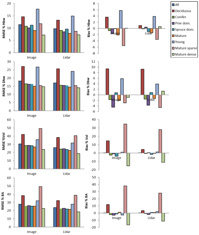
Fig. 2. RMSE in percent of mean and bias in percent of mean for mean height (Hbw), mean diameter (Dbw), stem volume (Vol) and basal area (BA) in different strata based on all plots for image and LiDAR models.
Image and LiDAR based models show in general similar performance for the different strata (Fig. 2); highest and lowest performance were predicted in same strata in both datasets. LiDAR based performance were always slightly better compared to images based performance. Hbw and Dbw were clearly overestimated in deciduous dominated forest and in young forests resulting in lower RMSE% compared to other strata. In addition Hbw was underestimated in mature sparse forests. Lowest accuracies for stem volume and basal area were produced in mature sparse, deciduous dominated and young forests, where deciduous dominated and mature sparse forests were clearly overestimated. Best performances were obtained in mature forests and especially in mature dense forests for all attributes, even though stem volume and basal area of mature dense forest was usually underestimated.
3.2 Stand level validation
Validating the models at stand level using all the validation stands (company and biotope combined) at each sub-area, the results are similar between the sub-areas except for Dbw in E2, where the RMSE was clearly higher (Table 6). For the best performing models of the sub-areas (E2, Q2 and R2), RMSE ranged from 7.7% to 10.5% for Hbw (E2 excluded); from 12.0% to 17.8% for Dbw; from 22.0% to 22.7% for stem volume; and from 17.7% to 21.1% for basal area. The bias for all variables in Q2 shows a rather large underestimation (from –5.0 to –9.6%). Fig. 3, shows that almost all stands with high stem volumes are underestimated in Q2, whereas in E2 and R2 volume estimates are more evenly distributed.
| Table 6. Stand level accuracies for basal area weighted mean height (Hbw), basal area weighted mean diameter (Dbw), stem volume (Vol), and basal area (BA) in different sub-areas (all stands). | ||||
| Dataset | Stand attribute | RMSE | RMSE (%) | Bias (%) |
| E2 | Hbw, m | - | - | - |
| Dbw, cm | 3.9 | 17.8 | –6.8 | |
| Vol, m3 ha–1 | 51.3 | 22.7 | 0.4 | |
| BA, m2 ha–1 | 4.6 | 17.7 | –3.6 | |
| Q2 | Hbw, m | 1.9 | 10.5 | –9.1 |
| Dbw, cm | 2.9 | 12.7 | –9.6 | |
| Vol, m3 ha–1 | 55.4 | 22.4 | –9.3 | |
| BA, m2 ha–1 | 4.6 | 18.6 | –5.0 | |
| R2 | Hbw, m | 1.5 | 7.7 | –0.4 |
| Dbw, cm | 3.1 | 12.0 | –5.3 | |
| Vol, m3 ha–1 | 57.4 | 22.0 | –6.7 | |
| BA, m2 ha–1 | 5.8 | 21.1 | –6.1 | |
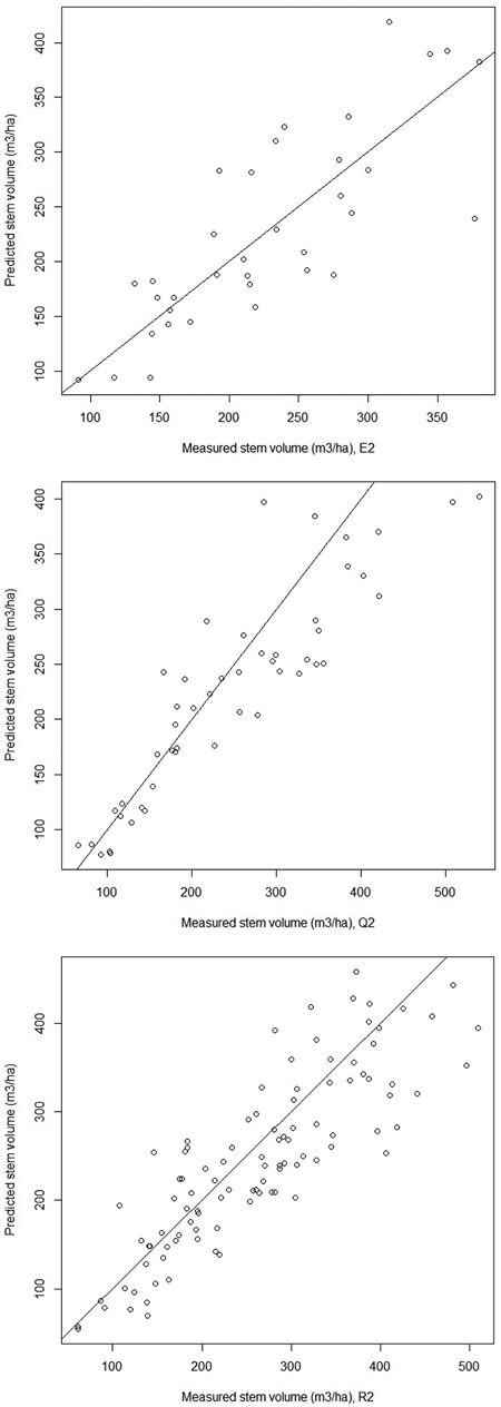
Fig. 3. Stand level stem volumes (m3 ha–1) in sub-areas; E2, Q2 and R2, based on field measurements and image data.
Stand data from all sub-areas were combined into one dataset of company stands, one dataset of biotope stands and one dataset of all stands and the model developed from each stands sub-area was applied to each stand, i.e., the best local model was used. In case of biotope stands and all stands, only accuracies of stem volume could be evaluated. Prediction accuracies are shown in Table 7. The relative RMSE for stem volume was better in biotope stands compared to company stands.
| Table 7. Stand level accuracies of forest attributes in combined datasets. Hbw = basal area weighted mean height and Dbw = basal area weighted mean diameter. | |||
| Characteristic | RMSE | RMSE (%) | Bias (%) |
| Company stands, n = 144 | |||
| Hbw, m | 1.6 | 8.6 | –5.6 |
| Dbw, cm | 2.7 | 11.0 | –5.6 |
| Basal area, m2 ha–1 | 5.3 | 20.2 | –5.4 |
| Stem volume, m3 ha–1 | 54.8 | 23.7 | –7.8 |
| Biotope stands, n = 39 | |||
| Stem volume, m3 ha–1 | 61.2 | 18.9 | –2.2 |
| All stands, n = 183 | |||
| Stem volume, m3 ha–1 | 55.7 | 22.2 | –6.1 |
Results applying models from different sub-areas to company stand of Q2 and R2 showed that stem volume model from sub-area E2 produced highest accuracies for both Q2 and R2, even higher than the model from the own sub-area (Table 8). In general, R2 model produced slightly poorer results than Q2 model for Q2, but both Q2 and R2 model produced equally good accuracies for R2. All models showed large bias for sub-area Q2 which is leaf-off.
| Table 8. RMSE% and Bias% of stem volume using models from different sub-areas to company stand of Q2 and R2. | ||
| Model-area | RMSE (%) | Bias (%) |
| Q2-Q2 | 23.0 | –11.5 |
| E2-Q2 | 19.2 | –8.3 |
| R2-Q2 | 25.3 | –17.3 |
| R2-R2 | 24.1 | 5.3 |
| E2-R2 | 22.4 | 0.9 |
| Q2-R2 | 24.6 | 2.0 |
4 Discussion
This study shows that 3D data from the standard aerial image acquisition carried out by Lantmäteriet together with training plots from the NFI can be used to estimate tree height, mean diameter, stem volume, and basal area for large areas. For forest production stands, the best results in terms of RMSE using these image data were 8.6% for tree height, 11.0 for mean diameter, 23.7% for stem volume, and 20.2% for basal area. For the Swedish national forest attribute map based on ALS data, stand wise accuracies for 253 forest production stands in south and mid Sweden, RMSE ranged from 5.4% to 9.5% for tree height; from 8.7% to 13.1% for stem diameter; from 17.2% to 22.0% for stem volume; from 13.9% to 18.2% for basal area (Nilsson et al. 2016). Both the result in this study and the reported accuracy of the current ALS based national forest attribute map are slightly lower than dedicated image- or LiDAR based inventories (Næsset et al. 2004; Gobakken et al. 2015). This may depend on factors like: i) poorer training plot positioning (Gobakken and Næsset 2009) i.e., NFI often uses raw GPS not DGPS as is common in remote sensing based inventories having positional errors of a few meters instead of sub-meter and ii) NFI uses a systematic sampling design compared to stratified designs commonly used in operational ALS based inventories (Maltamo et al. 2011).
The slightly lower accuracies for image based models, compared to LiDAR, can be missing information from within the forest canopy structure. When comparing stem volume estimates using point cloud metrics from LiDAR and metrics calculated from the CHM of the LiDAR data, relative RMSE at plot level increased from 31.5% to 35.5% (Hollaus et al. 2009), indicating that the information from within the canopy improves the accuracy of stem volume estimation. Also, a study comparing LiDAR and image metrics showed that many metrics differ between LiDAR and image based point clouds and that the difference increased with decreasing canopy cover (White et al. 2015). This indicates that image based data does not describe the gaps and height variance of the forest canopy as well as LiDAR. However, increasing the image overlap should theoretically decrease the occlusion by the surrounding trees of gaps and therefore increase the description of gaps and variance of the canopy height. But Bohlin et al. (2012) tested both 60/30 image overlap with 0.5 m GSD and 80/60 image overlap with 0.12 m GSD with no increase in estimation accuracy of stem volume.
The underestimation, –9.3%, for stem volume in Q2 (Table 6), is partly explained by a few high stem volume stands that has been underestimated (Fig. 3). Some of the high volume stands had large deciduous stem volume and Q2 images were acquired during leaf-off season, this affect the image matching to generate points mostly on the ground and with more noise and thus the canopy height metric values negatively (Véga and St-Onge 2008; Lisein et al. 2015; Bohlin et al. 2015), clearly underestimating raster cells with high deciduous proportion. Another reason for underestimation is that the mature stands, which are under estimated (Fig. 2), are over represented in the validation stand inventory due to the forest companies’ purpose of the inventory, resulting in that the performance of the models is not validated for the complete range of the models. However, the bias is similar to that reported for the ALS based national forest attribute map, i.e., 8.0–8.9%, 13.0–13.1%, 16.1–21.6% and 15.2–20.0% for Hbw, Dbw, BA and Vol respectively (Nilsson et al. 2016) , which have been widely used and is considered an important source of forest information.
Image and LiDAR based models show very similar trends of RMSE when performance is separated in different strata, indicating that both techniques have similar strength and weaknesses when it comes to estimate forest attributes in different forest types. This result is in agreement with a study from Canada where image and LiDAR based forest attributes were estimated for eight different forest types, and the accuracy varied for the different forest type but the overall accuracy between the two remote sensing methods were not statistically different (Pitt et al. 2014).
Comparing company and biotope stands, the biotope stands had higher estimation accuracy (Table 7), despite having higher proportion of deciduous trees. This may be an effect of the method used for field data collection, i.e., the company stands are sampled with a number of sample plots whereas in the biotope stands all trees are callipered, reducing the sampling error in the validation data. A large proportion of the estimation error in remote sensing based inventories validated at stand level with stands sampled by a number of plots can be because of the sampling error in the validation data (Lindgren 2012).
When models trained in other sub-areas were applied on Q2 and R2 validation stands, the E2 model was the best. The E2 training data has larger variation and might therefore better explain different forests than the local (sub-area) model. However, there is little difference between models. All models underestimated the stem volume in Q2 indicating that using leaf-on models on leaf-off data is not recommended as suggested for LiDAR based inventories (Villikka et al. 2012).
In ALS based forest inventories a stratified modelling approach is commonly used (Maltamo et al. 2014), where the training data is divided in to different strata based on auxiliary data e.g., height or density metric from the remotely sensed data, and separate models are constructed for each strata and forest attribute. This approach might also improve the accuracy for large-area mapping using aerial images and NFI data. Using the proposed method, an image block cover large enough area so that about 200 NFI plots can be utilized if two inventory years are used, preferably from the same year as the image acquisition and the year before.
5 Conclusion
Major advantages of this approach are the constant availability of new aerial images, the low cost of image data and no extra field data acquisition is need because of use of existing NFI data. Furthermore, Lantmäteriet has started to perform the stereophotogrammetry, i.e., producing 3D data, for all images acquired 2016 and onward as part of their annual image production, making it easy to implement the proposed method, as soon as point clouds of new image blocks are available and thus continuously updating the forest attribute map. However, the density of the forest is difficult to describe, which shows as a saturation of the estimation of high volumes as well as lower accuracies for volume and basal area compared to height and diameter. Further research must be aimed at investigating better describing density metrics as well as how the photogrammetric workflow e.g., image overlap and image matching method effect these metrics. Leaf-off season images has a large negative impact on the deciduous forest attribute estimations and is therefore not recommended. This study clearly shows that aerial images from the national image program together with sample plots from the National Forest Inventory can be used for large area forest attribute mapping.
Acknowledgments
The authors are grateful to the Swedish NFI, Bergvik Skog and the Swedish Forest Agency for providing field data. Special gratitude is directed to Lantmäteriet, which provided the R2 imagery. The authors are also grateful to the developers of R (R Core Team 2015), a free software environment for statistical computing and graphics, which was used for the statistical analyses. This work was financially supported by Formas and the Swedish Forest Agency. Finally we would like to thank the reviewers for their valuable comments.
References
Baltsavias E.P. (1999). A comparison between photogrammetry and laser scanning. ISPRS Journal of photogrammetry and Remote Sensing 54(2–3): 83–94. http://dx.doi.org/10.1016/S0924-2716(99)00014-3.
Bohlin J., Wallerman J., Fransson J.E.S. (2012). Forest variable estimation using photogrammetric matching of digital aerial images in combination with a high-resolution DEM. Scandinavian Journal of Forest Research 27(7): 692–699. http://dx.doi.org/10.1080/02827581.2012.686625.
Bohlin J., Wallerman J., Fransson J.E.S. (2015). Deciduous forest mapping using change detection of multi-temporal canopy height models from aerial images acquired at leaf-on and leaf-off conditions. Scandinavian Journal of Forest Research 31(5): 517–525. http://dx.doi.org/10.1080/02827581.2015.1130850.
Ginzler C., Hobi M.L. (2015). Countrywide stereo-image matching for updating digital surface models in the framework of the Swiss National Forest Inventory. Remote Sensing 7(4): 4343–4370. http://dx.doi.org/10.3390/rs70404343.
Gobakken T., Næsset E. (2009). Assessing effects of positioning errors and sample plot size on biophysical stand properties derived from airborne laser scanner data. Canadian Journal of Forest Research 39(5): 1036–1052. http://dx.doi.org/10.1139/X09-025.
Gobakken T., Bollandsås O.M., Næsset E. (2015). Comparing biophysical forest characteristics estimated from photogrammetric matching of aerial images and airborne laser scanning data. Scandinavian Journal of Forest Research 30(1): 73–86. http://dx.doi.org/10.1080/02827581.2014.961954.
Hijmans R.J. (2015). raster: Geographic data analysis and modeling. http://cran.r-project.org/package=raster.
Hirschmüller H. (2008). Stereo processing by semiglobal matching and mutual information. IEEE Transactions on Pattern Analysis and Machine Intelligence 30(2): 328–341. http://dx.doi.org/10.1109/TPAMI.2007.1166.
Hollaus M., Dorigo W., Wagner W., Schadauer K., Höfle B., Maier B. (2009). Operational wide-area stem volume estimation based on airborne laser scanning and national forest inventory data. International Journal of Remote Sensing 30(19): 5159–5175. http://dx.doi.org/10.1080/01431160903022894.
Honkavaara E., Markelin L., Rosnell T., Nurminen K. (2012). Influence of solar elevation in radiometric and geometric performance of multispectral photogrammetry. ISPRS Journal of Photogrammetry and Remote Sensing 67: 13–26. http://dx.doi.org/10.1016/j.isprsjprs.2011.10.001.
Korhonen L. Morsdorf F., (2014). Estimation of canopy cover, gap fraction and leaf area index with airborne laser scanning. In: Maltamo M., Næsset E., Vauhkonen J. (eds.). Forestry applications of airborne laser scanning. Managing Forest Ecosystems 27: 397–437. http://dx.doi.org/10.1007/978-94-017-8663-8.
Leberl F., Irschara A., Pock T., Meixner P., Gruber M., Scholz S., Wiechert A. (2010). Point clouds. Photogrammetric Engineering & Remote Sensing 10: 1123–1134. http://dx.doi.org/10.14358/PERS.76.10.1123.
Lindgren O. (2012). Validation of stand-wise forest data based on ALS. In: Full proceedings of SilviLaser 2012, first return, Sept. 16–19 September 2012, Vancover, Canda. Paper Number SL2012-014. 8 p.
Lisein J., Michez A., Claessens H., Lejeune P. (2015). Discrimination of deciduous tree species from time series of unmanned aerial system imagery. PLoS ONE 10(11): e0141006. http://dx.doi.org/10.1371/journal.pone.0141006.
Maltamo M., Bollandsas O.M., Naesset E., Gobakken T., Packalen P. (2011). Different plot selection strategies for field training data in ALS-assisted forest inventory. Forestry 84(1): 23–31. http://forestry.oxfordjournals.org/cgi/doi/10.1093/forestry/cpq039.
McGaughey R.J. (2015). FUSION/LDV: software for LIDAR data analysis and visualization. US Department of Agriculture, Forest Service, Pacific Northwest Research Station.
Næsset E. (2002). Predicting forest stand characteristics with airborne scanning laser using a practical two-stage procedure and field data. Remote Sensing of Environment 80(1): 88–99. http://dx.doi.org/10.1016/S0034-4257(01)00290-5.
Næsset E. (2014). Area-based inventory in Norway – from innovation to an operational reality. In: Maltamo M., Næsset E., Vauhkonen J. (eds.). Forestry applications of airborne laser scanning. Managing Forest Ecosystems 27: 215–240. http://dx.doi.org/10.1007/978-94-017-8663-8.
Næsset E., Gobakken T., Holmgren J., Hyyppä H., Hyyppä J., Maltamo M., Nilsson M., Olsson H., Persson Å., Söderman U. (2004). Laser scanning of forest resources: the nordic experience. Scandinavian Journal of Forest Research 19(6): 482–499. http://dx.doi.org/10.1080/02827580410019553.
Nilsson M., Nordkvist K., Jonzén J., Lindgren N., Axensten P., Wallerman J., Egberth M., Larsson S., Nilsson L., Eriksson J., Olsson H. (2016). A nationwide forest attribute map of Sweden predicted using airborne laser scanning data and field data from the National Forest Inventory. Remote Sensing of Environment. http://dx.doi.org/10.1016/j.rse.2016.10.022.
Nilsson P., Cory N., Kempe G., Fridman J. (2015). Skogsdata 2015, aktuella uppgifter om de svenska skogarna från Riksskogstaxeringen. Tema: Riksskogstaxeringens permanenta provytor. [Forest data 2015, current information about the Swedish forests from the National forest inventory. Theme: the National forest inventory’s permanent plots]. Official Statistics of Sweden, Swedish University of Agricultural Sciences, Umeå. http://pub.epsilon.slu.se/12626/.
Nord-Larsen T., Schumacher J. (2012). Estimation of forest resources from a country wide laser scanning survey and national forest inventory data. Remote Sensing of Environment 119: 148–157. http://dx.doi.org/10.1016/j.rse.2011.12.022.
Owemyr P, Lundgren J. (2010). Noggrannhetskontroll av laserdata för ny nationell höjdmodell. [Accuracy assesment of laser data for new national elevation model.] Master thesis, Högskolan i Gävle. Gävle, Sweden. http://www.diva-portal.org/smash/record.jsf?pid=diva2:444023.
Pitt D.G., Woods M., Penner M. (2014). A comparison of point clouds derived from stereo imagery and airborne laser scanning for the area-based estimation of forest inventory attributes in boreal Ontario. Canadian Journal of Remote Sensing 40(3): 214–232. http://dx.doi.org/10.1080/07038992.2014.958420.
R Core Team. (2015). R: a language and environment for statistical computing. R Foundation for Statistical Computing, Vienna, Austria. http://www.R-project.org/.
Rothermel M., Wenzel K., Fritsch D., Haala N. (2012). SURE: photogrammetric surface reconstruction from imagery. In: Proceeding of LC3D Workshop, Berlin, Germany. http://www.ifp.uni-stuttgart.de/publications/software/sure/index.en.html.
St-Onge B., Véga C., Fournier R.A., Hu Y. (2008). Mapping canopy height using a combination of digital stereo‐photogrammetry and lidar. International Journal of Remote Sensing 29(11): 3343–3364. http://dx.doi.org/10.1080/01431160701469040.
Tuominen S., Pitkänen J., Balazs A., Korhonen K., Hyvönen P., Muinonen E. (2014). NFI plots as complementary reference data in forest inventory based on airborne laser scanning and aerial photography in Finland. Silva Fennica 48(2) article 983. http://dx.doi.org/10.14214/sf.983.
Vastaranta M., Wulder M.A., White J.C., Pekkarinen A., Tuominen S., Ginzler C., Kankare V., Holopainen M., Hyyppä J., Hyyppä H. (2013). Airborne laser scanning and digital stereo imagery measures of forest structure: comparative results and implications to forest mapping and inventory update. Canadian Journal of Remote Sensing 39(5): 382–395. http://dx.doi.org/10.5589/m13-046.
Vauhkonen J., Maltamo M., McRoberts R.E., Næsset E. (2014). Introduction to forestry applications of airborne laser scanning. In: Maltamo M., Næsset E., Vauhkonen J. (eds.). Forestry applications of airborne laser scanning. Managing Forest Ecosystems 27: 1–16. http://dx.doi.org/10.1007/978-94-017-8663-8.
Véga C., St-Onge B. (2008). Height growth reconstruction of a boreal forest canopy over a period of 58 years using a combination of photogrammetric and lidar models. Remote Sensing of Environment 112(4): 1784–1794. http://dx.doi.org/10.1016/j.rse.2007.09.002.
Villikka M., Packalén P., Maltamo M. (2012). The suitability of leaf-off airborne laser scanning data in an area-based forest inventory of coniferous and deciduous trees. Silva Fennica 46(1): 99–110. http://dx.doi.org/10.14214/sf.68.
Waser L.T., Fischer C., Wang Z., Ginzler C. (2015). Wall-to-wall forest mapping based on digital surface models from image-based point clouds and a NFI forest definition. Forests 6(12): 4510–4528. http://dx.doi.org/10.3390/f6124386.
White J., Stepper C., Tompalski P., Coops N., Wulder M. (2015). Comparing ALS and image-based point cloud metrics and modelled forest inventory attributes in a complex coastal forest environment. Forests 6(10): 3704–3732. http://dx.doi.org/10.3390/f6103704.
White J.C., Wulder M.A., Varhola A., Vastaranta M., Coops N.C., Cook B.D., Pitt D.G., Woods M. (2013). A best practices guide for generating forest inventory attributes from airborne laser scanning data using an area-based approach. Natural Resources Canada, Canadian Forest Service, Canadian Wood Fibre Centre. http://cfs.nrcan.gc.ca/publications?id=34887.
White J.C., Wulder M.A., Vastaranta M., Coops N.C., Pitt D., Woods M. (2013). The utility of image-based point clouds for forest inventory: a comparison with airborne laser scanning. Forests 4(3): 518–536. http://dx.doi.org/10.3390/f4030518.
Wiechert A., Gruber M. (2011). UltraCam and UltraMap – towards all in one solution by photogrammetry. In: Fritsch D. (ed.). Photogrammetric week ’11. Wichmann/VDE Verlag, Belin & Offenbach. http://www.ifp.uni-stuttgart.de/publications/phowo11/050wiechert.pdf.
Total of 37 references.
Send to email
