Matti Maltamo  ,
Tomi Karjalainen,
Jaakko Repola,
Jari Vauhkonen
,
Tomi Karjalainen,
Jaakko Repola,
Jari Vauhkonen
Incorporating tree- and stand-level information on crown base height into multivariate forest management inventories based on airborne laser scanning
Maltamo M., Karjalainen T., Repola J., Vauhkonen J. (2018). Incorporating tree- and stand-level information on crown base height into multivariate forest management inventories based on airborne laser scanning. Silva Fennica vol. 52 no. 3 article id 10006. https://doi.org/10.14214/sf.10006
Highlights
- The most accurate tree-level alternative is to include crown base height (CBH) to nearest neighbour imputation
- Also mixed-effects models can be applied to predict CBH using tree attributes and airborne laser scanning (ALS) metrics
- CBH prediction can be included with an accuracy of 1–1.5 m to forest management inventory applications.
Abstract
This study examines the alternatives to include crown base height (CBH) predictions in operational forest inventories based on airborne laser scanning (ALS) data. We studied 265 field sample plots in a strongly pine-dominated area in northeastern Finland. The CBH prediction alternatives used area-based metrics of sparse ALS data to produce this attribute by means of: 1) Tree-level imputation based on the k-nearest neighbor (k-nn) method and full field-measured tree lists including CBH observations as reference data; 2) Tree-level mixed-effects model (LME) prediction based on tree diameter (DBH) and height and ALS metrics as predictors of the models; 3) Plot-level prediction based on analyzing the computational geometry and topology of the ALS point clouds; and 4) Plot-level regression analysis using average CBH observations of the plots for model fitting. The results showed that all of the methods predicted CBH with an accuracy of 1–1.5 m. The plot-level regression model was the most accurate alternative, although alternatives producing tree-level information may be more interesting for inventories aiming at forest management planning. For this purpose, k-nn approach is promising and it only requires that field measurements of CBH is added to the tree lists used as reference data. Alternatively, the LME-approach produced good results especially in the case of dominant trees.
Keywords
forest inventory;
LIDAR;
alpha shape;
crown height;
nearest neighbor;
mixed-effects model
-
Maltamo,
University of Eastern Finland, School of Forest Sciences, P.O. Box 111, FI-80101 Joensuu, Finland
E-mail
matti.maltamo@uef.fi
- Karjalainen, University of Eastern Finland, School of Forest Sciences, P.O. Box 111, FI-80101 Joensuu, Finland E-mail tomimkarjalainen@gmail.com
- Repola, Natural Resources Institute of Finland (Luke), Natural resources, Eteläranta 55, FI-96300 Rovaniemi, Finland E-mail jaakko.repola@luke.fi
- Vauhkonen, Natural Resources Institute of Finland (Luke), Bioeconomy and environment, Yliopistokatu 6, 80100 Joensuu, Finland E-mail jari.vauhkonen@luke.fi
Received 24 May 2018 Accepted 25 July 2018 Published 27 July 2018
Views 111929
Available at https://doi.org/10.14214/sf.10006 | Download PDF

1 Introduction
The size of a tree crown is an indicator of tree health, vigor, and growth and yield potential (Smith 1986; Salminen et al. 2005). The crown size is usually defined in terms of crown length, crown ratio, i.e., crown length divided by the total height of a tree, crown surface area or crown volume. Of those measures, crown length and crown ratio can be obtained most simply, because tree height is typically measured in forest inventories and only crown base height (CBH) needs to be measured in addition. The usability of CBH is not limited to crown size calculation: tree-level CBHs have been used to determine the quality classes and value of sawn logs (Uusitalo 1995; Verkasalo et al. 2004), and stand-level mean CBH can also be used to indicate on wood quality (Wall et al. 2004). CBH has also been used as a tree level predictor variable in tree growth (Salminen et al. 1995) and biomass component models (Repola 2009) and stand level predictor variable in fire behavior models (Andersen et al. 2005). CBH varies considerably between tree species being usually at a higher relative height for dominant species, such as Scots pine (Pinus sylvestris L.), and lower for shade tolerant species, such as Norway spruce (Picea abies [L.] H. Karst.). CBH is also related to silvicultural history, age and social status of a tree in a stand.
Information obtained by airborne laser scanning (ALS) is strongly related to some forest inventory attributes, such as tree height, different plot-level mean height characteristics, canopy cover and canopy gaps, and these attributes can be derived almost directly from the data (Naesset 2002; Thomas et al. 2008; Vepakomma et al. 2008; Korhonen et al. 2010). On the other hand, characteristics such as tree diameter distribution cannot be directly observed with ALS data and statistical relationships must be utilized to predict those (Gobakken and Naesset 2004).
Based on ALS data, the upmost surface of the tree crowns is typically described most accurately, since the first ALS echoes mainly reflect back from the top of the canopy. The description becomes less accurate towards the lower end of canopy, i.e., around the height of the crown base, because most of the first echoes have already reflected back and the subsequent echoes may suffer from transmission losses due to penetrating upper canopy. The challenges related to predicting CBH by ALS are further reviewed by Maguya (2015; Chapter 5) and at least three different prediction approaches can be distinguished based on earlier literature: First, some researchers have attempted to derive the CBH directly from the data, applying polygon, alpha shape or voxel based crown or canopy approximations (Pyysalo and Hyyppä 2002; Holmgren et al. 2008; Popescu and Zhao 2008; Vauhkonen 2010; Maltamo et al. 2010). Second, it may be possible to predict CBH according to descriptive statistics of ALS-based height value distribution without any statistical model (Solberg et al. 2006; Dean et al. 2009; Maltamo et al. 2010), especially when combined with expert opinion or calibration field data to indicate what statistics are relevant for the CBH. Third, using field data more integrally for model fitting, the relationships between ALS features and crown base height can be estimated using regression analysis or corresponding techniques (Naesset and Okland 2001; Andersen et al. 2005; Maltamo et al. 2006, 2010).
In Finland, ALS-based approaches have been established for the data acquisition of operational forest management inventories (Maltamo and Packalen 2014). Due to the requirements of the planning system, the inventory system must produce data at the tree-level, but practical accuracy and cost reasons prohibit the use of individual tree detection approaches. Instead, the practical forest inventories in Finland use area-based ALS data and k-nearest neighbor (k-NN) imputation to produce stand attributes such as mean diameter, dominant height, basal area and volume (for details, see Maltamo and Packalen 2014). Although the stand description is predicted at an area-level, the use of tree size distribution models transforms the description back to the tree-level, meaning that information of both tree and stand levels is available for the subsequent management or wood procurement planning. As reviewed above, it would benefit the aforementioned purposes, if also CBH predictions were available either at the tree or stand level. However, even though earlier studies have confirmed that such predictions are feasible based on available ALS data, there are no studies that would recommend on how this information should be linked to multivariate forest inventories, such as those described by Maltamo and Packalen (2014).
The aim of this study is to examine the possibilities to include crown base height prediction into multivariate forest inventory information using ALS. The study compares four different methods to predict the CBH, which can all be implemented with sparse ALS data and area-based metrics. The methods require different levels of field reference data and produce either tree or plot-level predictions. However, all methods are cross-validated at the plot-level, which corresponds to a scale where the aforementioned inventory systems are operated.
2 Material and methods
2.1 Study area and field data
The study area was located in Kuhmo, eastern Finland, and it was a combination of two separate laser scanning areas (Fig. 1). The Kuhmo region is very homogenous in terms of species, being strongly dominated by Scots pine. Also Norway spruces and deciduous trees, mainly birches (Betula spp.) and aspen (Populus tremula L.), are typically found, but especially the deciduous species usually form only minor proportions of suppressed trees.
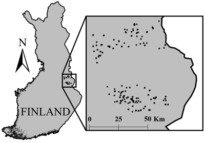
Fig. 1. The location of field sample plot clusters.
In this study, 265 field sample plots with co-located ALS and field data were available. The plots had been placed in L-shaped clusters of 5 plots according to old inventory data on development stages of forests in the area. The distance between plots in a cluster was 150 m. Every tree with a diameter at breast height (DBH) greater than 5 cm had been measured from the circular sample plots with a radius of 9 meters. The measured attributes were DBH, CBH, and species. Species-specific median trees of each plot, selected according to tree basal area, were measured for height. Tree-level basal areas were first calculated by formula π × (DBH/2)2 and the plot basal area (G) was summed from these measurements. The missing tree heights were predicted using Näslund’s (1936) height curve: On each plot, these curves were first calibrated using the height and DBH of the species-specific median trees (Siipilehto 1999). Tree stem volumes were estimated using Laasasenaho’s models (1982), which include the DBH, height and tree species as predictors. Pine and spruce had their own separate models and the model for birch was used in the case of all deciduous trees. The most essential characteristics of the studied plots are shown in Table 1.
| Table 1. The main attributes of the 265 studied field plots. Min = minimum, Max = maximum, Sd = Standard deviation. | |||||
| Attribute | Population | Mean | Min1 | Max | Sd |
| Volume (m3 ha–1) | Total | 124.2 | 1.42 | 403.3 | 78.3 |
| Scots pine | 88.8 | 0.45 | 294.2 | 61.7 | |
| Norway spruce | 39.2 | 0.19 | 400.6 | 55.8 | |
| Deciduous trees | 17.6 | 0.25 | 167.5 | 23.8 | |
| Basal area (m2 ha–1) | Total | 16.8 | 0.43 | 44.6 | 7.9 |
| Scots pine | 11.5 | 0.14 | 33.1 | 6.6 | |
| Norway spruce | 5.6 | 0.08 | 39.2 | 6.7 | |
| Deciduous trees | 2.8 | 0.08 | 18.7 | 3.2 | |
| Mean diameter (cm) | Total | 14.3 | 6.6 | 33.6 | 4.4 |
| Scots pine | 17.6 | 6.1 | 41.6 | 6.9 | |
| Norway spruce | 12.1 | 5.0 | 27.9 | 4.8 | |
| Deciduous trees | 10.8 | 5.1 | 44.6 | 5.4 | |
| Mean height (cm) | Total | 12.0 | 2.7 | 23.9 | 3.4 |
| Scots pine | 13.9 | 5.0 | 28.3 | 4.8 | |
| Norway spruce | 9.6 | 3.5 | 21.9 | 3.7 | |
| Deciduous trees | 10.6 | 2.7 | 23.6 | 4.0 | |
| Number of stems (ha–1) | Total | 1014 | 196 | 2790 | 507 |
| Scots pine | 538 | 39 | 1965 | 362 | |
| Norway spruce | 365 | 39 | 2476 | 401 | |
| Deciduous trees | 307 | 39 | 2397 | 308 | |
| Mean crown base height (dm) | Total | 48.9 | 8.7 | 129.6 | 21.0 |
| Scots pine | 67.3 | 8.8 | 189.3 | 34.1 | |
| Norway spruce | 20.1 | 3.0 | 62.6 | 13.5 | |
| Deciduous trees | 42.5 | 7.0 | 137.0 | 23.7 | |
| Basal-area-weighted mean crown base height (dm) | Total | 58.9 | 8.8 | 155.5 | 25.9 |
| Scots pine | 70.9 | 8.9 | 188.5 | 34.4 | |
| Norway spruce | 22.9 | 3.0 | 64.2 | 15.6 | |
| Deciduous trees | 46.4 | 7.0 | 142.4 | 26.9 | |
| 1 The Min-values present the smallest observations > 0, because all factually observed species-specific min-values would have been zeroes due to the absence of species in many plots (Scots pine was met on 246 plots, Norway spruce on 185 plots and deciduous trees on 218 plots). | |||||
The final study material consisted of 6527 trees, of which 3245 were Scots pines, 1661 Norway spruces and 1621 deciduous trees, the latter treated as a combined species group in this study. The pine proportion of stem number was therefore 49.7% and on average, pines were on dominant position in the stands and considerably larger than other tree species (Table 1).
Categorical forest characteristics measured from the plots included soil type, site type, development stage and dominant species (Table 2). According to this information, the plots represented widely different types of forests. Most of the plots had a mean DBH between 8 and 16 cm and could therefore by categorized as young stands, for which reason the mean CBHs were fairly low in the entire data (Table 1).
| Table 2. The distribution of plots according to categorical stand characteristics. DBH is the arithmetic mean of the DBH at the plot-level. The dominant species was determined as the species with the largest proportion from the sum of tree stem volumes in a plot. | |||
| Characteristic | Sub class | N | % |
| Soil type | Mineral soil | 201 | 75.8 |
| Peat soil | 64 | 24.2 | |
| Site type | Fertile / Oxalis-Myrtillus type (OMT) | 2 | 0.8 |
| Moderate / Vaccinium Myrtillus type (MT) | 181 | 68.3 | |
| Poor / Vaccinium vitis-idaea type (VT) | 82 | 30.9 | |
| Development class | T2 (DBH < 8 cm) | 8 | 3.0 |
| 02 (8 cm ≤ DBH < 16 cm) | 184 | 69.4 | |
| 03 (16 cm ≤ DBH < 24 cm) | 65 | 24.5 | |
| 04 (DBH ≥ 24 cm) | 8 | 3.0 | |
| Dominant species | Scots pine | 208 | 78.5 |
| Norway spruce | 42 | 15.8 | |
| Deciduous trees | 15 | 5.7 | |
2.2 ALS data
The study area was laser scanned from the air between 4th and 7th of September, 2011, when the deciduous trees still had their leaves on. The scanning was performed with Leica ALS50-II sensor from a flying altitude of 2000 m using a scanning angle of 30 degrees, scanning rate of 52 Hz and pulse frequency of 58.9 Hz. These parameters yielded a nominal data density of 0.52 pulses m–2. The data were acquired and pre-processed, including height normalization, by Arbonaut, Ltd. Height-normalized first echoes (”single” or “first-of-many”) of each pulse were extracted from the region of each plot. The ground threshold of 2 m was employed when computing the ALS features. Altogether 33 different plot-level ALS features were computed from the point data, including, i.e., percentiles and densities at relative heights 0.05; 0.1; 0.2,…, 0.9, 0.95 and central statistics of both the height and intensity values (Table 3).
| Table 3. The ALS metrics used in this study. Suffices single and first refer to using only single or first-of-many echoes, respectively; otherwise, the metrics were computed using pooled single and first-of-many echoes. | |
| ALS metric | Definition |
| CBHas | CBH prediction based on alpha shapes (see Section 2.3.3) |
| Hmax | Maximum height |
| Hmean | Mean height |
| Hstd | Standard deviation of height |
| Vegeratio | Ratio of the number of echoes above 2 m to the total number of echoes |
| H05…H95 | ith percentile of height |
| D05…D95 | Relative density at height i |
| Imean | Mean intensity |
| Imeansingle | Mean intensity (single echoes) |
| Imeanfirst | Mean intensity (first-of-many echoes) |
| Istd | Standard deviation of intensity |
| Istdsingle | Standard deviation of intensity (single echoes) |
| Istdfirst | Standard deviation of intensity (first-of-many echoes) |
| Prop_first | Proportion of first-of-many echoes |
2.3 Methods to predict crown base height
This study compared altogether four different methods that can be implemented with sparse, area-based ALS data. The methods however require different degrees of reference data in order to be run and therefore result to CBH predictions of different levels (tree or plot). The compared methods can be summarized according to the reference data requirements as follows:
1. Tree-level imputation requires that full field-measured tree lists including CBH observations are available for reference data.
2. Tree-level mixed-effects modelling approach requires similar reference data as alternative 1 for model fitting.
3. Plot-level prediction based on alpha shapes examines the properties of the point clouds for prediction and it can be applied without field information.
4. Plot-level regression analysis requires plot-level CBH observations for model fitting.
2.3.1 Tree-level imputation
The tree list imputation based on k-NN is fundamentally similar to Packalen and Maltamo (2008) and therefore referred to as PMk-NN. The idea is to search for k most similar plots in terms of chosen independent variables and to predict tree lists as weighted unions of trees measured from those plots, using the selected distance metric as the weights. The predicted tree lists, therefore, include all tree attributes available for each tree, being the species, DBH, height, and CBH in our case. The use of an imputation method requires choices on dependent and independent variables, distance metric, and a value of k within available training plot data (Maltamo et al. 2009), each of which affect the predictions (Latifi et al. 2010). These factors can be optimized with respect to desired accuracies in the training data (Packalen et al. 2012). As we focused on CBH, our PMk-NN was trimmed for these predictions, as explained below and further discussed in the Discussion section.
PMk-NN is based on the most similar neighbor (MSN) method, which employs canonical correlation analysis to produce a weighting matrix for selecting the NNs from the training data. Both the variable selection for the correlation analysis and the NN search were carried out in a leave-out-one-plot fashion using the yaImpute package (Crookston and Finley 2008) of the R statistical computing environment. The dependent (Y) and independent (X) variables were selected according to the Root Mean Squared Error (RMSE) of basal area weighted CBH with both k = 1 and k = 5, testing different variable combinations in two steps. First, the plot volume, basal area, the mean, minimum and maximum diameter and height, and 10th, 20th, ..., 90th percentiles of diameter and height distributions were tested one by one as the Y-variable, using all available ALS-features to form the vector of X-variables. The Y-variable that minimized the RMSEs was retained and new Y-variables were appended until the RMSE accuracy could not be improved. Then, the vector of Y-variables was fixed to that obtained above and the selection was repeated similarly for the X-variables. The sensitivity of both variable combinations was finally tested by replacing each selected X and Y variable with all possible non-selected candidates.
When predicting, the k parameter was set to be 5, meaning that the predicted tree-list of each plot was composed of the trees from 5 most similar plots. The CBH prediction of each plot was computed as the distance weighted mean of the CBHs measurements of the 5 plots. The relative weight w of individual plot i was calculated as:

where Di is the distance between the target and the plot i and n is the number of plots, in this case 5.
2.3.2 Tree-level mixed-effects model
In the tree-level modelling, the linear mixed-effects model (LME) was developed for predicting CBH of pine using tree DBH and height as the main predictors. In ALS-based forest inventory applications, the DBH and height are not known but they must first be predicted. Therefore, the constructed model was applied to the tree-lists produced by the PMk-NN method described above. Only the plots with pine as the dominant species were used as modeling data since mainly the dominant trees affect the plot-level ALS-metrics and our inventory area is strongly dominated by pine. The model included both the tree-level variables measured in the field and ALS-derived plot-level variables. The different ALS-derived variables such height percentiles (H05, H10, H20,…, H95), the densities value of each quantiles (D05, D10, D20,…, D95), ALS-based mean height and crown height were tested as plot-level independent variables (Table 3). To account for hierarchical data structure and obtain unbiased tests for variables at each level, the model was formulated as a linear mixed model (Searle 1987) with both fixed and random effects as follows:
![]()
where CBH is the response variable, a0 is the intercept, a and b are vectors of fixed regression coefficients, TREE is a vector of field measured tree characteristics for tree j in plot i, PLOT is a vector of ALS-based stand characteristics in plot i, ui is the random effect of plot i and eij is the residual error for tree j in plot i.
2.3.3 Plot-level prediction based on alpha shapes
The implementation of the alpha shape method (α-shape) corresponds precisely with the “Prediction alternative A” of Maltamo et al. (2010). It is based on examining geometrical and topological properties of the 3D point data to detect vertical gaps that distinguish canopy from the terrain and possible understorey shrubs. If such gaps exist and appear larger than within-canopy gaps in the ALS data, this method can detect the CBH directly from the point data and without any field work. According to the experiences of Maltamo et al. (2010), however, these predictions can be expected to include 20–40% more error compared to best ones obtained with field calibration data.
To implement this method, the plot-level ALS point clouds were intersected by a vector grid with a cell size of 4 × 4 m (Maltamo et al. 2010) to derive three-dimensional Delaunay triangulation and alpha shape (Edelsbrunner and Mücke 1994) based on the point data of each cell. CBHs were first predicted separately for each cell by filtering the alpha shapes according to parameter alpha, which can be considered as a size-criterion to determine the level of detail in the obtained triangulation (Vauhkonen 2010). The filtering started from such an alpha value that delimited the point cloud into one connected component representing canopy. The alpha values were traversed in descending order until a new component was split. The vertical position of each split component was examined relative to the initial component. The traversal of the alpha values was continued until new components located completely below the highest (canopy) component and above the ground threshold of 1 m could not be extracted. Cell-specific CBHs were defined as the heights of the lowest vertices in the filtered alpha shapes and plot-level predictions were obtained as their weighted averages, using the joint areas of the plot and cells as the weights.
2.3.4 Plot-level regression analysis
Linear regression (LR) analysis was used to construct a plot-level model separately for the arithmetic mean CBH and basal-area-weighted mean CBH. All the ALS variables available were used as candidate predictors in the model. The correlation between different predictors was tested with VIF-test (Variance Inflation Factor).
2.4 Validation
Plot-level validation was done separately for the whole data and for subsets of plots with the proportions of tree species groups ≥ 50% of the total volume. Altogether 201, 38 and 15 plots were dominated by Scots pine, Norway spruce and deciduous tree species, respectively. The remaining 11 plots without a clear dominant species were classified as mixed stands. We wanted to evaluate the predictions of these plots separately, because it is known that the CBH is a tree species dependent attribute. We considered both arithmetic mean CBH and basal-area-weighted mean CBH (cf. Eqs. 3–4): using PMk-NN and LME methods, also the predicted plot-level CBH was either an arithmetic mean or weighted by the basal area obtained from the tree lists. When validating the predictions, a leave-one-plot-out cross-validation (LOOCV) was applied to all predictions except those produced by alpha shapes, which did not require model fitting or calibration. The validation was based on the root mean squared error (RMSE, Eq. 3) and mean difference (BIAS, Eq. 4)

and

where y is the observed plot-level arithmetic or basal-area-weighted mean CBH, x is the predicted plot-level mean CBH and n is the number of plots. Using PMk-NN, LME and LR, also the predicted CBH was either arithmetic mean or the basal-area-weighted mean. The Relative RMSEs and biases were calculated by multiplying the absolute values with factor 100/y, where y is the average CBH in the population studied.
3 Results
3.1 Constructed models
3.1.1 Tree-level imputation
Altogether three X- and three Y-variables were used for the PMk-NN imputation (Table 4). In the first step of the feature selection, the RMSE of both k = 1 and k = 5 was improved by including the minimum and 70th percentile of tree heights and the 80th percentile of tree diameters as Y-variables. Two candidate Y-variables would still have improved the result with k = 1, but less than 1% in terms of the RMSE-improvement compared to using three Y-variables. All these candidates also increased the RMSE with k = 5, for which reason the first step of the feature selection was terminated. In the second step, Hmean, D90, and H10 were selected as X-variables. With k = 5, altogether 12 additional X-variables would have provided similar decimal-level improvements to the RMSE and one of the candidate X-variables as much as 5%, compared to the last variable added. All of these variables however increased the RMSE with k = 1, for which reason the second step of the feature selection was terminated. Adding or removing Y-features did not improve the RMSE compared to the combination presented in Table 4.
| Table 4. Features selected for the tree list imputations. The RMSEs refers to those of basal-area weighted plot-level mean CBHs and the Impr. columns give the improvement in RMSE (%) compared to the previous step. | ||||||
| Step | X-feature(s) | Y-feature(s) | RMSE | RMSE | ||
| k = 1 | Impr. | k = 5 | Impr. | |||
| 1 | All | Heightmin | 3.11 | - | 2.77 | - |
| All | Heightmin + Height70 | 1.59 | 49.04 | 1.42 | 48.58 | |
| All | Heightmin + Height70 + Diameter80 | 1.54 | 2.59 | 1.36 | 4.24 | |
| 2 | Hmean | Heightmin + Height70 + Diameter80 | 1.47 | 4.95 | 1.34 | 1.49 |
| Hmean + D90 | Heightmin + Height70 + Diameter80 | 1.30 | 11.19 | 1.23 | 7.97 | |
| Hmean + D90 + H10 | Heightmin + Height70 + Diameter80 | 1.30 | 0.57 | 1.23 | 0.38 | |
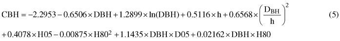
3.1.2 Tree level mixed-effects model
The constructed mixed-effect model for CBH was based on field-measured tree diameter at breast height (DBH) and tree height (h), and ALS-derived variables such 5th and 80th percentiles of height (H05, H80) and the relative density at the relative height of 0.05 (D05). In addition to the main effect of these variables, DBH was used also as interaction term with h, D05 and H80. All the independent variables were highly significant i.e. the p-value was < 0.0001, except ln(DBH) with p-value of 0.0011. The final mixed-effect model was specified as follows:
The error variance was 0.843 m between plots and 1.328 m between trees, meaning that from the unexplained residual variance, a greater part occurred between trees then between plots – furthermore meaning that the model was actually more accurate predicting plot-level mean CBH than the CBH of a single tree.
3.1.3 Plot level linear regression model
The significance (p-value) of each predictor was examined and the least significant candidate was removed from the model. This procedure was repeated until the p-value of each predictor was smaller than 0.001. The final combination of predictors was manually chosen from this group by minimizing the RMSE. Additionally, to avoid multicollinearity, VIF-value greater than 5 between two predictors was not allowed. Different transformations were also tested but they did not improve neither the model accuracy nor the plotted residuals.
The final form of the linear regression model for predicting the arithmetic mean crown base height (CBHARI) was the following (Eq. 6):
![]()
where Hstd is the standard deviation of the height, H10 is the 10th percentile of height, D50 is the relative density at the relative height 0.5 and Imean_all is the mean of intensities. The error variance and adjusted R-square of the model were 1.1 m and 0.72, respectively, in the entire data. However, using the LOOCV approach in the validation calculations changed the variance and coefficient values above between the iterations.
Correspondingly, the final form of the linear regression model for predicting the basal-area- weighted crown base height (CBHBAW) was the following (Eq. 7):
![]()
where D20 is the relative density at the relative height 0.2. The error variance and adjusted R-square were 1.2 m and 0.78, respectively, in the entire data.
3.2 Plot-level reliability figures
The RMSEs and biases observed for the different methods are shown in the Table 5 for the whole study data. The relative RMSEs were always lower for the basal-area-weighted mean crown base height (CBHBAW ) than for the arithmetic mean crown base height (CBHARI) , where the improvement is because of the increase in the reference CBH value due to the basal-area weighting.
| Table 5. The RMSEs and biases obtained with different methods when predicting the plot-level arithmetic mean crown base height (CBHARI) or basal-area-weighted mean crown base height (CBHBAW) for the whole study data. | ||||
| CBHARI | PMk-NN | LME-model | α-shape | LR-model |
| RMSE (dm) | 12.65 | 15.61 | 16.42 | 11.29 |
| %-RMSE | 25.89 | 31.95 | 33.59 | 23.10 |
| BIAS (dm) | –0.64 | –8.43 | –9.67 | –0.01 |
| %-BIAS | –1.30 | –17.25 | –19.79 | –0.02 |
| CBHBAW | ||||
| RMSE (dm) | 14.47 | 17.42 | 15.16 | 12.29 |
| %-RMSE | 24.59 | 29.60 | 25.76 | 20.89 |
| BIAS (dm) | 1.05 | –8.91 | 0.31 | 0.02 |
| %-BIAS | 1.78 | –15.13 | 0.53 | 0.03 |
The linear regression model was the most accurate alternative for both CBHARI and CBHBAW. It is not surprising, since it modelled the plot-level mean CBH using straightforward regression analysis. In that case, predictions matching closely with the reference values could be obtained without bias. The RMSEs were 0.11–0.12 m.
The PMk-NN method showed the second best accuracy figures. The imputation of tree-level CBH values also turned out to be more accurate than applying the LME-model to the PMk-NN-produced tree lists. The LME-model in particular led to considerably high overestimates.
The alpha shape method was the least accurate alternative to predict CBH in the case of the arithmetic mean, although it did not perform remarkably poorly compared to the other methods. In the case of the basal-area-weighted mean CBH, the accuracy of the alpha shape method was better than that of the LME-model and almost as good as for the PMk-NN-method. The alpha shape method also overestimated the CBH even more than the LME-model in the case of the arithmetic mean, but was almost unbiased toward the basal-area-weighted values.
The reliability figures of both the arithmetic and basal-area-weighted CBH are additionally shown for plots dominated by the different species (Tables 6 and 7). The reliability figures were in general better in the pine-dominated plots and especially for the LME-model. Also the bias values were lower. This is an obvious result, since the LME-model was originally constructed at the tree-level using observations of pine plots only. In the case of basal-area-weighted mean CBH, the LME-model was even more accurate than the PMk-NN approach in pine plots (Table 7). As above, the reliability figures of the alpha shape method were better for basal-area-weighted mean CBH values. The alpha shape method was interestingly more accurate than PMk-NN in the spruce plots. Additionally in the plots dominated by spruce, the reliability figures varied depending on the method and whether the evaluation was done with respect to the arithmetic or basal-area-weighted mean CBH. Only for deciduous plots, the CBH predictions were always poor (considerable overestimates), which may be due to the fact that the reference CBH values were generally lower for these plots.
| Table 6. The RMSEs and biases obtained with different methods when predicting the plot-level arithmetic mean CBH for the plots dominated by different species or mixed plots. | ||||
| Scots pine (n = 201) | PMk-NN | LME-model | α-shape | LR-model |
| RMSE (dm) | 12.71 | 14.00 | 15.55 | 11.14 |
| %-RMSE | 24.68 | 27.19 | 30.21 | 21.63 |
| BIAS (dm) | 1.10 | –6.25 | –8.50 | 0.79 |
| %-BIAS | 2.14 | –12.14 | –16.52 | 1.53 |
| Norway spruce (n = 38) | ||||
| RMSE (dm) | 9.32 | 17.48 | 14.11 | 7.97 |
| %-RMSE | 20.86 | 39.12 | 31.57 | 17.83 |
| BIAS (dm) | –2.71 | –13.93 | –9.66 | 0.19 |
| %-BIAS | –6.07 | –31.17 | –21.62 | 0.42 |
| Deciduous species (n = 15) | ||||
| RMSE (dm) | 18.93 | 27.63 | 29.21 | 16.88 |
| %-RMSE | 55.66 | 81.24 | 85.90 | 49.64 |
| BIAS (dm) | –13.68 | –20.46 | –22.46 | –8.34 |
| %-BIAS | –40.23 | –60.15 | –66.03 | –24.55 |
| Mixed (n = 11) | ||||
| RMSE (dm) | 10.88 | 13.98 | 14.81 | 7.60 |
| %-RMSE | 30.50 | 39.19 | 41.51 | 21.29 |
| BIAS (dm) | –7.41 | –12.76 | –13.58 | –3.67 |
| %-BIAS | –20.78 | –35.75 | –38.08 | –10.30 |
| Table 7. The RMSEs and biases obtained with different methods when predicting the plot-level basal-area-weighted mean CBH for the plots dominated by different species or mixed plots . | ||||
| Scots pine (n = 201) | PMk-NN | LME-model | α-shape | LR-model |
| RMSE (dm) | 13.88 | 12.81 | 14.72 | 11.54 |
| %-RMSE | 22.31 | 20.58 | 23.66 | 18.54 |
| BIAS (dm) | 4.34 | –4.58 | 2.24 | 2.20 |
| %-BIAS | 6.97 | –7.36 | 3.60 | 3.53 |
| Norway spruce (n = 38) | ||||
| RMSE (dm) | 14.04 | 26.33 | 13.38 | 11.63 |
| %-RMSE | 26.04 | 48.84 | 24.82 | 21.57 |
| BIAS (dm) | –6.80 | –22.86 | –0.45 | –5.94 |
| %-BIAS | –12.61 | –42.39 | –0.83 | –11.02 |
| Deciduous species (n = 15) | ||||
| RMSE (dm) | 21.28 | 33.07 | 24.12 | 21.04 |
| %-RMSE | 55.80 | 86.74 | 63.26 | 55.19 |
| BIAS (dm) | –14.95 | –24.82 | –18.34 | –9.66 |
| %-BIAS | –39.20 | –65.11 | –48.12 | –25.33 |
| Mixed (n = 11) | ||||
| RMSE (dm) | 14.99 | 20.67 | 12.73 | 11.72 |
| %-RMSE | 35.27 | 48.67 | 29.98 | 27.59 |
| BIAS (dm) | –10.15 | –18.07 | –6.79 | –5.95 |
| %-BIAS | –23.89 | –42.54 | –15.98 | –14.02 |
Finally, the residuals of predicting the arithmetic mean CBH and basal-area-weighted mean CBH using the compared methods are shown in Figs. 2 and 3, respectively. In general, the residuals were evenly distributed. However, especially the LME-model and alpha shape method generally overestimated the CBH values of the plots not dominated by pine. Figs. 2 and 3 also provide more background for the biased reliability figures of those methods.
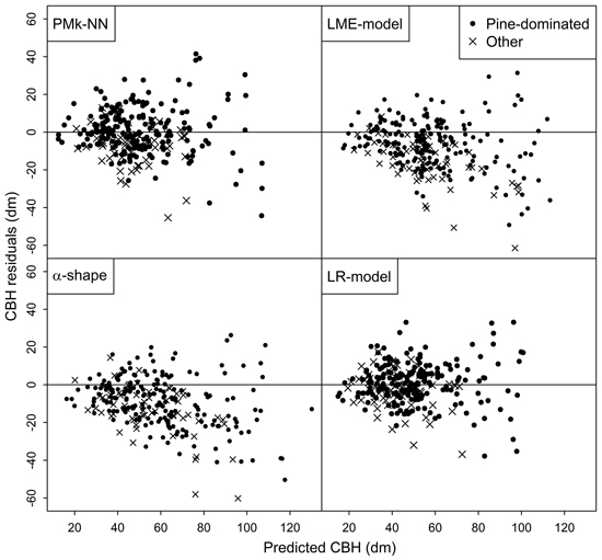
Fig. 2. Residuals of the different methods in the prediction of arithmetic mean CBH.
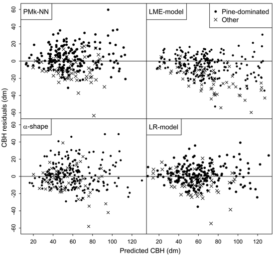
Fig. 3. Residuals of the different methods in the prediction of basal-area-weighted mean CBH.
4 Discussion
This study considered the prediction of CBH using sparse density ALS data. The plot-level validation showed that CBH can be predicted in most cases at an accuracy of about 1–1.5 meters for plots dominated by different species. Only for plots with deciduous trees, the error values were considerably higher. The results above can be regarded as promising in that all of the tested methods can be feasibly applied in ALS based large scale forest inventory. The observed relative RMSEs were between 21% and 34% in the whole data and between 18% and 30% in the pine dominated plots (i.e., the most frequent and the most important species of the inventory area). These values are somewhat high compared to RMSEs reported earlier (Maltamo et al. 2010). However, the reason may be related to generally low reference CBH values, when even a minor absolute error may result to high relative figures. Another reason for the low relative accuracy may be the aforementioned wide distribution of development classes from saplings to mature stands on the plots studied (Table 2). For comparison, Maltamo et al. (2010) focused on mature Norway spruce stands and reported RMSEs of approximately 13–20% on independent validation plots.
The use of PMk-NN based trees list is an appropriate alternative for generating tree-level CBHs in ALS based forest inventory. Tree level estimates can be directly used in different models (biomass, tree growth) and these estimates can be flexible aggregated to desired units such as stands. The reliability of this approach was almost always better than that of the LME alternative and the estimates were also almost unbiased in the whole data and pine dominated plots. Since k-nn is already used in ALS based forest inventories (Hudak et al. 2008; Maltamo and Packalen 2014) the inclusion of crown base height as a target variable only requires that it is measured from field plots in each inventory project similar to DBH and tree height are currently measured. The development of field measurement devices, especially different altimeters, may allow taking measurements for CBH together with those for the tree heights. However, the feasibility of measuring tree-level CBHs in the field depends, on one hand, on the costs related to the measurements and, on the other hand, on the benefits of including this attribute in the description of the tree stock.
It should be noted that the current tree lists of the PMk-NN method were produced using independent and dependent variables selected to predict CBH values as well as possible. Many other possibilities for training the nearest neighbor search exist and different combinations of features representing both the tree- and plot-levels could be used (Packalen et al. 2012; Vauhkonen et al. 2014). The tree lists used in our study may therefore represent best-case accuracies for CBH predictions. However, it should be noted that also earlier studies optimized the composition of the tree lists specifically for the variables used in evaluation. Additionally, in k-nn analyses the weighting of different tree attributes must be re-solved if new attributes are added as dependent variables. In practice, however, we acknowledge that less accurate CBH predictions are possibly obtained based on tree lists optimized for other purposes such as predicting tree diameter and height distributions accurately.
The use of the mixed-effects model with both the tree and stand level predictors led to almost as good RMSE values as the PMk-NN imputation in the whole data. However, the estimates were biased at the plot-level. There are two possible sources for the bias. First, the DBH and height used with the mixed-effects model were those obtained from the PMk-NN tree lists. Since this approach was optimized for predicting CBH, the other tree attribute estimates might not be as accurate as possible (see above discussion). We examined the accuracy and precision of the LME approach in more detail from this point of view by examining the residuals of the CBHs against the mean DBH and height predicted for the plots (detailed results not shown). The trend between the residuals of these attributes was, indeed, stronger in the case of the LME model predictions than those obtained from the PMk-NN tree lists. However, although the plots with high residual errors based on the PMk-NN method had inaccurate DBH and height, the LME model was not found to magnify the CBH errors in these plots.
More importantly, the LME-model was constructed by using only pine-dominated plots but applied to plots including all species. This choice is reflected from the better plot-level reliability figures for the pine-dominated plots, but poorer estimates for the plots dominated by the other species. Using the models fundamentally assumes that the predictions are always made for target stands having pine trees in the dominant canopy layer, which was reasoned in the present case due to the strong dominance of Scots pine in the inventory area. If applied in another study area with different species composition, the plots dominated by different species should be distinguished from each other based on the ALS data. Even though certain plot-level intensity metrics derived from sparse ALS point clouds were found to differ between dominant species in another study area dominated by Scots pine (Vauhkonen et al. 2014), the use of similar metrics to distinguish between dominant species was only moderately successful in the presently available data (Räty et al. 2016). As discussed in more detail by Räty et al. (2016), the reason could be related to the fact that the intensity recordings were not range-corrected and no flying trajectory data to perform the calibration were available. We cannot thus rule out the possibility that if range-corrected, some intensity metrics could possibly have been selected more often also to the presently formulated models. Yet, it would be difficult to envisage considerable accuracy improvements due to such a calibration. We also experimented a model version which included all trees but the model reliability was worse due to the high number of suppressed trees (the bias increased 0.1 m in the modelling data). Overall, our mixed-effects model is more useful for predicting tree-level CBHs as an indicator of stand-level saw log quality than producing tree crown information for the whole tree stock.
Direct plot-level estimates of canopy base height were also included. Although the accuracy of these alpha shape estimates was the worst among the compared methods in the case of arithmetic mean CBH values, it should be noted that this estimate can be obtained directly from the ALS point cloud without field data. On the other hand, these predictions were almost unbiased for the whole study area and pine and spruce plots, when evaluated against the basal-area-weighted mean values, indicating a better quantification of the properties related to the largest trees of the stands. On the other hand, the considerable overestimation of the arithmetic CBH could also indicate on either that the direct detection of vertical gaps is overly sensitive for within-canopy gaps in the upper canopy, or that the ALS point cloud is not sufficiently dense from the lower parts (Korhonen et al. 2013). Notably, the approach cannot even theoretically produce the lowest reference CBHs because of the ground threshold applied. In the studied data, there were two plots with mean CBH below this threshold (1 m). Interestingly, the alpha shape approach showed better accuracies for spruce-dominated plots and the approach overall performed better in the spruce-dominated study area of Maltamo et al. (2010), which may jointly imply a need for a data-specific calibration. Finally, the alpha shape estimate was never included in the models or PMk-NN neighbor search, even if being available as a candidate predictor.
The plot-level regression estimate was the most accurate alternative also showing the best-case accuracy that can be obtained for plot-level mean CBH predictions in this data set using ALS. On the other hand, a separate model must be constructed each time for different reference values, as in this study when using either the arithmetic or basal-area weighted mean CBH. Including the plot-level estimates of CBH in multivariate forest inventories may improve the possibilities to calibrate the estimates using similar techniques as in Kotivuori et al. (2018). On the other hand, it is also possible to transfer mixed-effect models effectively by means of local calibration using a low number of measurements either within an inventory area (Maltamo et al. 2012) or between inventory areas, even at the national scale (Kotivuori et al. 2016).
In this study the prediction of CBH was examined at the plot-level. However, if CBH estimation is included to ALS based multivariate forest inventory the interest and benefit of the approach is especially in species-specific-estimates. Since our study area was strongly dominated by one species, the number of plots (n = 265) was rather low for multivariate forest inventory and we only had ALS data, which are not feasible conditions for species-level analyses. The results presented here for pine dominated plots, however, show that for the dominant species, this metric can be predicted adequately. Therefore, further work is proposed to examine the reliability of species level CBH estimates.
5 Conclusions
The study showed that tree-level crown base height prediction can be included with an accuracy of 1–1.5 m to forest management inventory applications based on sparse ALS data. The most obvious alternative is to add tree-level CBH information to training data of k-nn imputation in addition to typically used species, DBH and height. As a result, wall-to-wall estimates of these attributes can be obtained. This study showed that k-nn approach is the most accurate tree-level alternative for CBH modelling and it can be preferred also due to the potential to provide tree-level predictions, the quality of which should however be further verified. Alternatively, mixed-effects models can be applied to predict CBH using tree attributes and plot-level ALS metrics. The benefit of the mixed-effects modeling approach is that once the model is formulated, it can be applied in other areas without new training data. Additionally, it can also be calibrated with rather low number of local measurements.
Acknowledgements
The study was funded by the project “Puuston laatutunnusten mittaus ja mallinnus” of Ministry of Agriculture and Forestry of Finland. The authors would like to thank Metsähallitus and Arbonaut Oy Ltd for providing study materials.
References
Andersen H.E., McGaughey R.J., Reutebuch S.E. (2005). Estimating forest canopy fuel parameters using LIDAR data. Remote Sensing of Environment 94(4): 441–449. http://dx.doi.org/10.1016/j.rse.2004.10.013.
Crookston N.L., Finley A. (2008). yaImpute: an R package for kNN imputation. Journal of Statistical Software 23(10). 16 p. http://dx.doi.org/10.18637/jss.v023.i10.
Dean T.J., Cao Q.V., Roberts S.D., Evans D.L. (2009). Measuring heights to crown base and crown median with LiDAR in a mature, even-aged loblolly pine stand. Forest Ecology & Management 257(1): 126–133. http://dx.doi.org/10.1016/j.foreco.2008.08.024.
Edelsbrunner H., Mücke E.P. (1994). Three-dimensional alpha shapes. ACM Transactions on Graphics 13(1): 43–72. http://dx.doi.org/10.1145/174462.156635.
Gobakken T., Naesset E. (2004). Estimation of diameter and basal area distributions in coniferous forest by means of airborne laser scanner data. Scandinavian Journal of Forest Research 19(6): 529–542.
Holmgren J., Persson Å., Söderman U. (2008). Species identification of individual trees by combining high resolution LIDAR data with multi-spectral images. International Journal of Remote Sensing 29(5): 1537–1552. http://dx.doi.org/10.1080/01431160701736471.
Hudak A.T., Crookston N.L., Evans J.S., Hall D.E., Falkowski M.J. (2008). Nearest neighbor imputation of species-level, plot-scale forest structure attributes from LiDAR data. Remote Sensing of Environment 112(5): 2232–2245. http://dx.doi.org/10.1016/j.rse.2007.10.009.
Korhonen L., Korpela I., Heiskanen J., Maltamo M. (2011). Estimation of vertical canopy cover and angular canopy gap fraction with airborne laser scanning. Remote Sensing of Environment 115(4): 1065–1080. http://dx.doi.org/10.1016/j.rse.2010.12.011.
Korhonen L., Vauhkonen J., Virolainen A., Hovi A., Korpela I. (2013). Estimation of tree crown volume from airborne lidar data using computational geometry. International Journal of Remote Sensing 34(20): 7236–7248. http://dx.doi.org/10.1080/01431161.2013.817715.
Kotivuori E., Korhonen L., Packalen P. (2016). Nationwide airborne laser scanning based models for volume, biomass and dominant height in Finland. Silva Fennica 50(4) article 1567. http://dx.doi.org/10.14214/sf.1567.
Kotivuori E., Maltamo M. Korhonen L., Packalen P. (2018). Calibration of nationwide airborne laser scanning based stem volume models. Remote Sensing of Environment 210: 179–192. http://dx.doi.org/10.1016/j.rse.2018.02.069.
Laasasenaho J. (1982). Taper curve and volume functions for pine, spruce and birch. Communicationes Instituti Forestalis Fenniae 108. 74 p. http://urn.fi/URN:ISBN:951-40-0589-9.
Latifi H., Nothdurft A., Koch B. (2010). Non-parametric prediction and mapping of standing timber volume and biomass in a temperate forest: applications of multiple optical/LiDAR-derived predictors. Forestry 83(4): 395–407. http://dx.doi.org/10.1093/forestry/cpq022.
Maguya A.S. (2015). Use of airborne laser scanner data in demanding forest conditions. Doctoral thesis, Lappeenranta University of Technology, Lappeenranta, Finland. Acta Universitatis Lappeenrantaensis, Volume 683. http://urn.fi/URN:ISBN:978-952-265-903-3. [Cited 7 March 2018].
Maltamo M., Hyyppä J., Malinen J. (2006). A comparative study of the use of laser scanner data and field measurements in the prediction of crown height in boreal forests. Scandinavian Journal of Forest Research 21(3): 231–238. http://dx.doi.org/10.1080/02827580600700353.
Maltamo M., Packalén P., Suvanto A., Korhonen K.T., Mehtätalo L., Hyvönen P. (2009). Combining ALS and NFI training data for forest management planning; a case study in Kuortane, Western Finland. European Journal of Forest Research 128(3): 305–317. http://dx.doi.org/10.1007/s10342-009-0266-6.
Maltamo M., Bollandsås O.M., Vauhkonen J., Breidenbach J., Gobakken T., Næsset E. (2010). Comparing different methods for prediction of mean crown height in Norway spruce stands using airborne laser scanner data. Forestry 83(3): 257–268. http://dx.doi.org/10.1093/forestry/cpq008.
Maltamo M., Mehtätalo L., Vauhkonen J., Packalén P. (2012). Predicting and calibrating tree size and quality attributes by means of airborne laser scanning and field measurements. Canadian Journal of Forest Research 42(11): 1896–1907. http://dx.doi.org/10.1139/x2012-134.
Maltamo M., Packalen P. (2014). Species specific management inventory in Finland. In: Maltamo M., Naesset E., Vauhkonen J. (eds.). Forestry applications of airborne laser scanning – concepts and case studies. Managing Forest Ecosystems vol. 27, Springer. p. 241–252. http://dx.doi.org/10.1007/978-94-017-8663-8_12.
Næsset E. (2002). Predicting forest stand characteristics with airborne scanning laser using a practical two-stage procedure and field data. Remote Sensing of Environment 80(1): 88–99. http://dx.doi.org/10.1016/S0034-4257(01)00290-5.
Næsset E., Økland T. (2002). Estimating tree height and tree crown properties using airborne scanning laser in a boreal nature reserve. Remote Sensing of Environment 79(1): 105–115. http://dx.doi.org/10.1016/S0034-4257(01)00243-7.
Packalén P., Maltamo M. (2008). The estimation of species-specific diameter distributions using airborne laser scanning and aerial photographs. Canadian Journal of Forest Research 38(7): 1750–1760. http://dx.doi.org/10.1139/X08-037.
Packalen P., Temesgen H., Maltamo M. (2012). Variable selection strategies for nearest neighbor imputation methods used in remote sensing based forest inventory. Canadian Journal of Remote Sensing 38(5): 557–569. http://dx.doi.org/10.5589/m12-046.
Popescu S.C., Zhao K. (2008). A voxel-based lidar method for estimating crown base height for deciduous and pine trees. Remote Sensing of Environment 112(3): 767–781. http://dx.doi.org/10.1016/j.rse.2007.06.011.
Pyysalo U., Hyyppä H. (2002). Reconstructing tree crowns from laser scanner data for feature extraction. International Archives of Photogrammetty and Remote Sensing. Spatial Information Science XXXIV Part 3B: 218–221.
Räty J., Vauhkonen J., Maltamo M., Tokola T. (2016). On the potential to predetermine dominant tree species based on sparse-density airborne laser scanning data for improving subsequent predictions of species-specific timber volumes. Forest Ecosystems 3(1). 17 p. http://dx.doi.org/10.1186/s40663-016-0060-0.
Repola J. (2009). Biomass equations for Scots pine and Norway spruce in Finland. Silva Fennica 43(4): 625–647. http://dx.doi.org/10.14214/sf.184.
Salminen H., Lehtonen M., Hynynen J. (2005). Reusing legacy FORTRAN in the MOTTI growth and yield simulator. Computational Electronics in Agriculture 49(1): 103–113. http://dx.doi.org/10.1016/j.compag.2005.02.005.
Smith D.M. (1986). The practice of silviculture. 8th edn. New York John Wiley and Sons, Inc. 527 p.
Solberg S., Næsset E., Bollandsås O.M. (2006). Single tree segmentation using airborne laser scanning data in a structurally heterogeneous spruce forest. Photogrammetric Engineering & Remote Sensing 72: 1369–1378. http://dx.doi.org/10.14358/PERS.72.12.1369.
Thomas V., Oliver R.D., Lim K., Woods M. (2008). Lidar and Weibull modeling of diameter and basal area. Forestry Chronicle 84(6): 866–875. http://dx.doi.org/10.5558/tfc84866-6.
Uusitalo J. (1995). Pre-harvest measurement of pine stands for sawing production planning. University of Helsinki, Department of Forest Resource Management, Publications 9.
Vepakomma U., St-Onge B., Kneeshaw D. (2008). Spatially explicit characterization of boreal forest gap dynamics using multi-temporal lidar data. Remote Sensing of Environment 112(5): 2326–2340. http://dx.doi.org/10.1016/j.rse.2007.10.001.
Verkasalo E., Sairanen P., Kilpeläinen H., Maltamo M. (2004). Modelling the end-use based value of Norway spruce trees and logs by using predictors of stand and tree levels. In: Nepveu G. (ed.). Connection between forest resources and wood quality: modelling approaches and simulation software. Proceedings of the fourth workshop, September 8–15, 2002. Harrison Hot Springs, British Columbia, Canada. p. 474–488.
Wall T., Fröblom J., Kilpeläinen H., Lindblad J., Heikkilä A., Song T., Stöd R., Verkasalo E. (2004). Harvennusmännyn hankinnan ja sahauksen kehittäminen. [Developing the procurement and sawing of thinned scots pine trees]. Wood Wisdom – tutkimusohjelman hankekonsortion julkinen loppuraportti. Laaja versio. [In Finnish]. Finnish Forest Research Institute, Joensuu Research Unit, Joensuu, Finland.
Vauhkonen J. (2010). Estimating crown base height for Scots pine by means of the 3D geometry of airborne laser scanning data. International Journal of Remote Sensing 31(5): 1213–1226. http://dx.doi.org/10.1080/01431160903380615.
Vauhkonen J., Packalen P., Malinen J., Pitkänen J., Maltamo M. (2014). Airborne laser scanning based decision support for wood procurement planning. Scandinavian Journal of Forest Research 29(S1): 132–143. http://dx.doi.org/10.1080/02827581.2013.813063.
Total of 37 references.
