Ilkka Korpela  ,
Antti Polvivaara,
Saija Papunen,
Laura Jaakkola,
Noora Tienaho,
Johannes Uotila,
Tuomas Puputti,
Aleksi Flyktman
,
Antti Polvivaara,
Saija Papunen,
Laura Jaakkola,
Noora Tienaho,
Johannes Uotila,
Tuomas Puputti,
Aleksi Flyktman
Airborne dual-wavelength waveform LiDAR improves species classification accuracy of boreal broadleaved and coniferous trees
Korpela I., Polvivaara A., Papunen S., Jaakkola L., Tienaho N., Uotila J., Puputti T., Flyktman A. (2023). Airborne dual-wavelength waveform LiDAR improves species classification accuracy of boreal broadleaved and coniferous trees. Silva Fennica vol. 56 no. 4 article id 22007. https://doi.org/10.14214/sf.22007
Highlights
- First study to assess dual-wavelength waveform data in tree species identification
- New findings regarding waveform features of previously unstudied species
- Waveform features correlated with tree size displaying wavelength- and species-specific differences linked to bark reflectance, height growth rate and foliage density
- Effects by pulse length and beam divergence are highlighted.
Abstract
Tree species identification constitutes a bottleneck in remote sensing applications. Waveform LiDAR has been shown to offer potential over discrete-return observations, and we assessed if the combination of two-wavelength waveform data can lead to further improvements. A total of 2532 trees representing seven living and dead conifer and deciduous species classes found in Hyytiälä forests in southern Finland were included in the experiments. LiDAR data was acquired by two single-wavelength sensors. The 1064-nm and 1550-nm data were radiometrically corrected to enable range-normalization using the radar equation. Pulses were traced through the canopy, and by applying 3D crown models, the return waveforms were assigned to individual trees. Crown models and a terrain model enabled a further split of the waveforms to strata representing the crown, understory and ground segments. Different geometric and radiometric waveform attributes were extracted per return pulse and aggregated to tree-level mean and standard deviation features. We analyzed the effect of tree size on the features, the correlation between features and the between-species differences of the waveform features. Feature importance for species classification was derived using F-test and the Random Forest algorithm. Classification tests showed significant improvement in overall accuracy (74→83% with 7 classes, 88→91% with 4 classes) when the 1064-nm and 1550-nm features were merged. Most features were not invariant to tree size, and the dependencies differed between species and LiDAR wavelength. The differences were likely driven by factors such as bark reflectance, height growth induced structural changes near the treetop as well as foliage density in old trees.
Keywords
crown modeling;
laser scanning;
photogrammetry;
individual tree detection;
Scandinavia
-
Korpela,
University of Helsinki, Department of Forest Sciences, P.O. Box 27, FI-00014 University of Helsinki, Finland
 0000-0002-1665-3984
E-mail
ilkka.korpela@helsinki.fi
0000-0002-1665-3984
E-mail
ilkka.korpela@helsinki.fi
- Polvivaara, University of Helsinki, Department of Forest Sciences, P.O. Box 27, FI-00014 University of Helsinki, Finland
-
Papunen,
University of Helsinki, Department of Forest Sciences, P.O. Box 27, FI-00014 University of Helsinki, Finland
0000-0001-5383-4314
E-mail
saija.papunen@outlook.com
- Jaakkola, University of Helsinki, Department of Forest Sciences, P.O. Box 27, FI-00014 University of Helsinki, Finland E-mail laura.jaakkola@helsinki.fi
-
Tienaho,
University of Eastern Finland, Faculty of Science and Forestry, P.O. Box 111, FI-80101 Joensuu, Finland
0000-0002-6574-5797
E-mail
noora.tienaho@uef.fi
- Uotila, University of Helsinki, Department of Forest Sciences, P.O. Box 27, FI-00014 University of Helsinki, Finland E-mail johannes.uotila@helsinki.fi
-
Puputti,
University of Helsinki, Department of Forest Sciences, P.O. Box 27, FI-00014 University of Helsinki, Finland
0000-0003-1972-1636
E-mail
tuomas.puputti@helsinki.fi
-
Flyktman,
University of Helsinki, Department of Forest Sciences, P.O. Box 27, FI-00014 University of Helsinki, Finland
0000-0002-5235-317X
E-mail
aleksi.flyktman@helsinki.fi
Received 7 September 2022 Accepted 13 January 2023 Published 26 January 2023
Views 84692
Available at https://doi.org/10.14214/sf.22007 | Download PDF

1 Introduction
Airborne LiDAR data are used for many purposes, and the justifications for the present study originate from LiDAR remote sensing (RS) of forests (Vauhkonen et al. 2014). It has for example, become an essential part of forest management planning systems in Finland (Maltamo and Packalén 2014). LiDAR is an observation tool that has reduced the sampling intensity and provided entirely new observations for the estimation of tree and forest attributes. In Finland, forest planning inventories use a combination of field reference, aerial image and LiDAR data, all finally followed by a field inspection. The data acquisition costs have been reduced compared with field-work intensive systems, with both enhancements and deficiencies in the deliverables. The primary deficiency in forest RS, not only in Finland, is tree species identification (Fassnacht et al. 2016). Information about the tree species is, however, crucial on technical, economic and ecological grounds. Thus, there is a need for enhanced observations and interpretation methods.
There are complexities that limit the accuracy achievable in tree species identification using both passive optical and LiDAR RS. In closed canopies, only the dominant trees are visible to the sensor with a high probability, which is a major weakness for many end users. Discriminating features are scale-specific and often exhibit large within-species variation. Atmospheric effects, illumination conditions, mixing of background signals, and directional effects cause further signal variation in passive imaging (Pisek et al. 2010; Koukal and Atzberger 2012). In LiDAR, atmospheric attenuation influences the signals, but the monostatic configuration of LiDAR reduces the directional effects into one dimension only (incidence angle) and the signals by the forest floor do not mix with the canopy. Also, the role of atmospheric scattering of sunlight is insignificant except for daytime single-photon LiDAR sensing (Swatantran et al. 2016).
Regarding airborne sensors, foresters have mostly used data acquired by topographic discrete-return (DR) small-footprint instruments that operate on a single wavelength. Narrow beams of small-footprint sensors promote accurate geometry and reach the ground. A pulsed LiDAR sensor transmits a short pulse of collimated light (typically some nanoseconds in duration) that illuminates targets on its path. The returning photon surge (time-dependent signal) that enters the receiver’s aperture is a convolution of the transmitted pulse with the backscatter-cross section profile of the targets (incl. multiple scattering). The receiver’s impulse response influences the detected analogue signal while digitization noise impacts further the sampled waveform (WF), if the receiver is designed to sample and store it (Wagner et al. 2006; Wagner 2010). Receivers in DR sensors analyze the signal on-the-fly for range data (individual echoes) and do not store the WF. The use of DR data has dominated, but many DR sensors can sample and record the return WF using optional circuits (Hovi 2015, p. 16). A WF consists of amplitudes values that are sampled at high frequency, for example, at intervals of one nanosecond, which corresponds to a one-way LiDAR−target range of 0.15 m.
WFs extend the information content of DR data as they reveal the measurement process of a pulsed LiDAR (Lim et al. 2003; Roncat et al. 2014; Anderson et al. 2016). WFs were shown to be beneficial for tree species identification (Reitberger et al. 2008; Yu et al. 2014; Hovi et al. 2016). While simulation studies have emphasized how sensor properties impact the available information (Disney et al. 2010; Hovi and Korpela 2013), certain limitations pertain to sensor design. They include the need for extremely high dynamic range, consideration of eye safety, receiver sensitivity and bandwidth, availability of powerful lasers at different wavelengths, data transfer and storage capacity requirements, weight and power consumption, limitations on the size of the mirror and the aperture, and the final instrument cost. Recent advances relate to improvements in productivity (an increase of pulse repetition frequency and/or flying height) by using sensors that combine several fast and sensitive scanners or by using so-called single-photon systems (White et al. 2021). Modern sensors can detect up to 10−12 echoes per transmitted pulse, and there are lightweight sensors for unmanned vehicles (Hu et al. 2020). DR systems that combine three scanners operating at different wavelengths (532, 1064 and 1550 nm) were made available for the experimenters and have shown potential in species identification (Kukkonen et al. 2019).
Both DR and waveform-recording pulsed airborne LiDAR data have been applied in tree species classification (Holmgren and Persson 2004; Reitberger et al. 2008; Korpela et al. 2010; Yao et al. 2012; Hovi et al. 2016; Blomley et al. 2017; Kukkonen et al. 2019; Rana et al. 2022). The features that characterize tree species were mostly found using a data-driven approach. Simulators that utilize realistic geometric-optical models of trees could, in principle, be used for finding optimal features, sensors and acquisition settings, but experimental case studies have prevailed. In airborne LiDAR, features that have been found to discriminate species measure implicitly crown shape, branching pattern, foliage density, gap size distribution, leaf orientation and overall reflectance properties of the canopy. Tree height and crown length are ‘directly’ measurable in LiDAR and can also guide species classification. In DR data, the predictor variables (features) are derived using 3D points observations with an associated ‘intensity’ observation. When using WF data, more features are available to characterize the trees. In both DR and WF cases, the information content of a single pulse is limited due to noise, and species classification has relied on distribution metrics derived from several pulses per tree.
In this study we explore the option of using dual-wavelength LiDAR for tree species identification. Wavelength impacts the WFs if the targets’ directional optical properties depend on the wavelength. Soft targets such as tree crowns consist of directional gaps and optically varying surfaces that vary in orientation, density, size, and spatial arrangement (Mallet and Bretar 2009; Roncat et al. 2014; Hancock et al. 2015). A combination of non-correlating wavelengths will therefore carry more information about the target, as shown in tree species identification by Danson et al. (2018) and Kukkonen et al. (2019). In Finland, findings by Hovi (2015, p. 33) suggested that the three main tree species show a different relative response in WF peak amplitude between 1064 and 1550 nm, but the combination of these wavelengths has not been tried thus far using WF data. Examining the influence of the wavelength on the WFs in trees would ideally incorporate sensors and data acquisitions settings that eliminate the influence of all other factors, such as the length of the transmitted pulse, footprint size (beam divergence), the receiver’s impulse response and sensitivity, signal-to-noise ratio (SNR), or scan zenith angle (Wagner 2006; Hovi and Korpela 2013; Korpela 2017; Korpela et al. 2020). For example, Kukkonen et al. (2019) used a three-band DR sensor in species classification, which showed poor performance of 532-nm metrics, which was due to a very low SNR of that band in the used sensor.
In the present study, we examined WFs by two single-band sensors that operate on the wavelengths of 1064 and 1550 nm. Sensor properties other than the wavelength differed somewhat between the sensors and needed to be accounted for in the interpretation of the results. The analyses were done at the tree-level by assigning pulses to individual trees. Our specific objectives were:
1) to find species-specific traits in 1064-nm and 1550-nm WF features of seven tree species classes that include living coniferous and broadleaved species and dead-standing Norway spruce,
2) to examine the correlation of WF features between the sensors (wavelengths) and the correlation of WF features with tree age,
3) to assess the gain from using dual-wavelength WF data in tree species identification.
2 Materials and methods
2.1 Study area and auxiliary data
The experiment was conducted in Hyytiälä, Finland (61.85°N, 24.29°E). The forests are dominated by Scots pine (Pinus sylvestris L.) (hereafter referred to as pine) and Norway spruce (Picea abies (L.) H. Karst.) (hereafter referred to as spruce). Birch (silver and downy birch combined; Betula pendula Roth, B. pubescens Ehrh.) occurs mainly as a mixed species. These are the main tree species in Finland. Other species were European aspen (Populus tremula L.), black alder (Alnus glutinosa (L.) Gaertn.) and Siberian larch (Larix sibirica Lebed.). These species are hereafter referred to as aspen, alder and larch. The age structure of Hyytiälä forests is shaped by a clear-cut regime that began in 1950 and has favored pine and spruce. Birch was planted only after 1972. Deciduous trees are in full leaf from late May until mid-September. Depending on the site quality, pine and spruce attain heights of 21−33 m at the age of 100 years, while the growth of birch is slightly faster. Dominant trees were not harvested in intermediate fellings. As a result, the tree height of dominant trees correlates strongly with stand age. Elevation varies moderately (140–195 m above sea level). There have been systematic aerial imaging and laser scanning campaigns since 1985 and 2004, respectively. All images have been oriented (see Korpela 2006) using bundle block adjustment to sub-pixel accuracy. We used RGB and color-infrared images in 10−20-cm resolution from 11/2011, 7/2012 and 5/2013 in the photogrammetric tasks as well as a LiDAR elevation model in 1-m resolution, which has an elevation accuracy of better than 20 cm.
2.2 LiDAR data
2.2.1 Acquisition dates and vegetation phenology
We had two LiDAR datasets (Table 1) from May 28, 2013, and June 16, 2013, when the temperature sum was 200- and 400-degree days, respectively. Campaigns took place in clear sky conditions, and dry weather prevailed in the preceding days of both acquisitions. New shoots in pine and spruce had started their growth the previous week to the first campaign, and while birch and alder were in full leaf, leaves were not entirely developed in some of the aspen clones. Pine stamens were ‘blooming’ during the first acquisition.
| Table 1. Parameters of the LiDAR data sets. | ||
| Scanner | Riegl LMS-Q680i | Leica ALS60 |
| Wavelength, nm | 1550 | 1064 |
| Date | May 28, 2013 | June 16, 2013 |
| Pulse repetition frequency, Hz | 240 | 106 |
| FWHM, transmitted pulse, ns | 4.5 | 7.8 |
| Pulse density p×m–2 | 12−20 | 10 |
| Flying height, m | 750 | 700 |
| Flying speed, m×s–1 | 41 | 62 |
| Strip overlap, % | 75 | 55 |
| Scan angle, ±° | 30 | 15 |
| Footprint diameter (86%), cm | 36 | 16 |
| WF samples per pulse | n × 80 | 1 × 256 |
| WF sampling rate, GHz | 1 | 1 |
| Discrete returns per pulse | 1−10 | 1−4 |
2.2.2 Geometric processing and accuracy
Geometric preprocessing of both datasets included strip matching and range calibration and resulted in pulse records with attributes for i) the 3D position of the sensor, ii) the 3D direction vector of the pulse, iii) the range between the sensor and the first recorded WF amplitude in meters (considering convolution with a hard target) and iv) file pointers to WF segments stored in binary files. The 3D accuracy (68%) of pulse paths was 25 cm or better and was assessed using power lines and GNSS-measured road profiles. The geometric processing was essential to enable accurate tracing of the transmitted pulses in the scene. Aerial images in Hyytiälä are oriented using a network of signaled ground control points (<0.05 m), and the systematic offsets between image blocks and LiDAR point clouds have been below 0.3 m.
2.2.3 Differences in WF storage between sensors
LMS-Q680i saves a WF sample of the transmitted pulse, and the received WF consisted of 1−3 sequences with 80, 160, 240 or 320 amplitude values. There can be pauses between sequences if the backscattering dims between the canopy and the ground. The separate WF sequences were merged into a contiguous WF, and the no-data gaps were filled with zeroes. Merging merely simplified the algorithms as the ALS60 WFs were always contiguous 256-nanosecond-long recordings. LMS-Q680i is a ‘genuine’ full-waveform sensor (Ullrich and Pfennigbauer 2011), whereas ALS60 is primarily a DR sensor, and our sensor had the optional oscilloscopes (WDM65) that sample the return WF only, not the transmitted WF. Both sensors applied a threshold, i.e. the return signal needs to exceed a certain threshold to start the WF storage. The sensors were compared by Korpela et al. (2013), and the peak amplitude of the return WFs correlated strongly in both sensors with the silhouette area of coniferous shoots that filled the footprint. In LMS-Q680i, we estimated that the threshold was exceeded by green foliage (1550-nm reflectance of 0.3) that fills 3−4% of the footprint area and is located in the center of the footprint, where the power is the largest.
2.2.4 Range normalization and radiometric corrections
ALS60 applies a variable receiver gain (0−3 dB), whereas Riegl Q680i has a different design for expanding the dynamic range of the sensor. It hosts two signal channels that differ by 6 dB in gain. We used the more sensitive channel, and these amplitude data were in a linear correlation with the factory-calibrated DR intensity values. The low-gain channel is intended for very strong return signals, and we observed that some ground returns were distorted in the high-gain channel, but the distortion was not observed in trees. The distortion causes bias in echo width estimates. This was observed in low-altitude (300 m AGL) data in an open peatland near Hyytiälä (Korpela et al. 2020). That data was captured during the same day with the same LMS-Q680i sensor.
Successful range-normalization of spherical losses using the radar equation requires that the WF amplitude values correspond to ratio scale observations of instantaneous received power (Wagner 2006). Range-normalization is important for improving the precision of WF features of individual trees that are computed from pulses arriving from several directions. Our range-normalization was a simple multiplication of each amplitude with the term (R/Rref)×(R/Rref), where R is the range and Rref was 700 m (Ahokas et al. 2006). With ±30° scan angle variation and ±25 m elevation variation, quadratic losses caused the return power to vary ±20% in the LMS-Q680i data (in extended targets). In ALS60, the variation of the scan angle was lower, ±15°, but the lower flying height increased the relative effect by the varying terrain elevation. In LMS-Q680i data, an offset term of 2 was subtracted from the observed amplitude values before range-normalization to have the amplitude data on the ratio scale (observations in powerline cables were used for the estimation of the offset term) and the small (0−10%) influence of the varying receiver gain (AGC circuit) in ALS60 was compensated with a polynomial model by Korpela (2017) that uses gain values stored in the data. The amplitude scale of the ALS60 sensor was deemed nearly linear (Korpela 2017), and an offset of 11.7 was subtracted from the raw amplitude values. This offset was estimated in that study using repeated scans from 700, 800 and 900 m acquisition heights. These calibration scans were a part of the same 2013 LiDAR campaign that we used in the present study. Thus, the calibration is valid for the present study.
2.2.5 Properties of the WFs
Both sensors recorded amplitude data at one-nanosecond intervals i.e. at ‘distances’ of 15 cm. Fig. 1 shows ‘two-return WFs’ of pulses that reflected first from a horizontal (football goal’s) crossbar 2.5 m above ground followed by a ground return in the grass. LMS-Q680i return pulses are symmetric with an FWHM (full-width-half-maximum) echo width of 4.5 ns. ALS60 pulses are longer (7.8 ns) and have a gradual tail end. The peaks (bar−ground) have a separation of 17−19 ns, which is 2.5−2.9 m in range. As expected, the pulse arriving at the 27-degree zenith angle shows the largest bar-ground distance. The examples in Fig. 1 illustrate why LMS-Q680i (1550 nm) WFs display more details in vegetation compared to ALS60 (1064 nm). In LMS-Q680i, a 10−12-ns-long buffer starts each WF sequence, while the length of the buffer in ALS60 WFs was 25−30 ns. In vegetation, the buffers of both sensors showed occasionally weak backscattering (branch), which had not (yet) triggered the recording but was stored and visible in the buffer. Fig. 2 illustrates how the return echoes widen when the target’s backscatter cross-section profile extends in depth. This occurs commonly in soft volumetric targets such as vegetation.
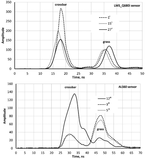
Fig. 1. Sample waveforms (WFs) of three LMS680i and three ALS60 pulses intersecting a football goal’s crossbar (height 2.5 m) and grass. The scan zenith angles (SZAs) are marked in degrees. WF sequences start with a buffer of amplitude values that display the signal prior to the storage-triggering echo. Their length is approximately 12 and 20 nanoseconds in the two sensors. The WF peaks (crossbar–grass) are separated more in the oblique pulse with an SZA of 27° compared to the vertical pulse (SZA = 1°). Return pulses of LMS-Q680i are symmetric, whereas ALS60 return pulses display ‘a tail’ even in hard targets. The asymmetry is due to the shutter in the laser transmitter that closes ‘slowly’.
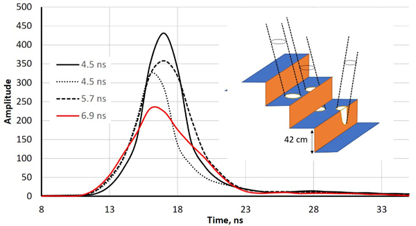
Fig. 2. Illustration of echo-widening in the LMS-Q680i. The four return waveforms are from wooden benches with a 42-cm vertical spacing. Echo widths (defined as full-width- half-maximum, FWHM) range from 4.5 ns to 6.9 ns. The width was 4.5 ns for pulses that illuminated a single planar surface. The pulse that displayed a 6.9-ns echo width intersected two bench layers, and the 5.3-ns pulse likely also illuminated the vertical part of the structure (illustrated by the drawing with three pulses).
2.3 Reference trees
We used trees of two field plots and additional trees, which were positioned (by LiDAR monoplotting, see Fig. 1 in Korpela et al. 2009) using visual interpretation of high-resolution image and LiDAR data. Fig. 3 shows the map of reference trees (n = 2532). Field plots ‘Old Growth’ (OG, 1.1 ha, N61.8314°, E24.3082°) and ‘Intermediate’ (IM, 0.7 ha, N61.8346°, E24.3181°) represent mature 100−125-yr-old and 45−50-yr-old trees, respectively (Fig. 4). Plots were established using a protocol in which treetops of dominant trees are first positioned in airborne data and later in the field using triangulation and trilateration (Korpela et al. 2007). Field measurements were carried out in 2015 and 2013, and stem DBH and crown status were observed for all trees. In these plots and in similar campaigns, the species classification accuracy of visual interpretation has been 97−99% when using multiple high-resolution images (10−20 cm) per tree. To increase the sample size of birch and to include more age variation in the other species, we measured additional 30−150-year-old pines, spruces, dead (standing) spruces and birches near the field plots using visual interpretation. These trees represent dominant and co-dominant trees with heights of 10−34 m (Fig. 5). To include rare species, samples of aspen, black alder and larch were also measured in images. Alders (17−25 m) are from two planted stands which had field mapped trees to support image interpretation, and most larches (13−32 m) are from five 25−100-yr-old stands. Aspen (13−31 m) is rare and occurs in small clones, which were identified in leaf-off aerial images of 2011, in which the bright bark and branching pattern were distinct features that supported visual interpretation (Fig. 6). We had a priori information about the locations of aspen clones from a local forester. In total, there were seven species classes: pine (n = 491), spruce (n = 801), dead spruce (n = 187), birch (n = 423), aspen (n = 167), alder (n = 148) and larch (n = 365).
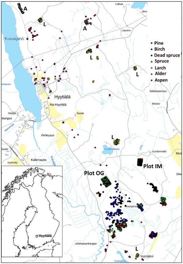
Fig. 3. Map of reference trees in Hyytiälä (61°49´N, 24°18´E), Finland. Field plots OG and IM are marked separately on the map, as well as the larch (L), and alder (A) stands. The map shows an area of 3×5 km.

Fig. 4. Stem diameter(dbh)×height distributions of trees in field plots IM and OG.

Fig. 5. Height distributions of trees measured in aerial images. Dead refers to dead spruce.
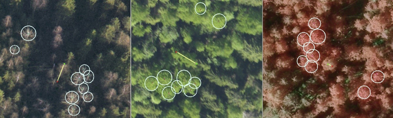
Fig. 6. Example of visual multi-image interpretation with 9 aspen crowns detected in leaf-off and leaf-on images captured in 11/2011 (left), 5/2013 (middle) and 6/2012 (right). The line segments show the ‘stem’ of a 24-m-high birch, which is used as the center point. The other ‘greyish’ trees in the leaf-off image are birches, and the green crowns are spruces.
2.4 Crown envelope models
To assign WF sequences to each tree, we applied crown models (Eq. 1, Fig. 7) that predict the crown radius at a given relative height (Korpela et al. 2011). The operator viewed multiple aerial images and pointed the tree’s apex in one to measure the 3D coordinates by monoplotting. Given height and species, an approximate envelope model was computed first and was then refined (weighted least squares regression) to the point cloud data. The operator altered iteratively the expected values of the model parameters until the model fitted the point cloud and crown in the image. The model was:
![]()
where a, b and c are the model parameters, x is the relative distance (0−1) down from the treetop, and rcrown is the radius of the crown in meters. For example, if the treetop of a 27-m-high tree was at the elevation (Z) of 172.70 m and the parameter values of this tree were c = 0.099, b = 0.642, and a = 0.564, the crown radius 5 m below the top (at Z = 167.20 m) is computed using x = 5/27, and the radius is 1.47 m.
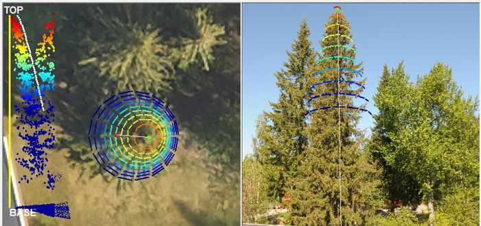
Fig. 7. Illustration of crown modeling of an urban Norway spruce. Aerial image on the left has the target tree in the middle with the current solution of the crown model superimposed as a colored wireframe graph. Terrestrial image on the right was taken from the roof of a building and was included here for illustration only. The graph in the left part of the aerial image shows the stem (yellow line) connecting the treetop and the base. The colored points are the LiDAR points near the tree. Their x-coordinate is the horizontal distance to the stem. Returns from the neighboring spruce are visible in the colored point cloud.
2.5 Assigning pulses and WF sequences to trees
Each tree was searched for pulses that potentially intersected the crown. The process is illustrated in Fig. 8. Given the crown model and the geometry of each pulse, it was possible to compute pulse-crown and pulse-ground intersections in 3D. These were used for splitting the return WF into segments representing separately the crown, understory, and ground. Because of the convolution, the segments were defined to have some overlap near Pexit and PGround (Fig. 8), as we did not carry out explicit WF decomposition (Roncat et al. 2014) into discrete returns. For example, WFGround in Q680i data was assigned amplitude values ±1.2 m from the ground, corresponding to a sequence of 17−18 amplitude values. In ALS60, the ground segment was defined PGround ±1.8 m owing to the longer transmitted pulses (Fig. 9). Because real crowns are not circular symmetric smooth surfaces, there were many pulses near the outer perimeter of the crowns, which mathematically intersected the crown model, but showed no backscattering and were thus rejected. Oblique pulses could show backscattering preceding Penter due to a neighboring tree or a single distinct branch. It is evident that the labeling of pulses is not free from errors, but the 3D delineation, despite its computational burden, results in minimal labeling errors. In order to simplify the computations, we assumed a fixed 40% crown ratio, which is a compromise as crown length depends on the species and stand history. It is likely that the crown models were too short for spruces growing in sparse stands, while the models exaggerate the crown length of densely grown pine and birch. The XYZ coordinates of a WF amplitude were defined by a time offset (distance along the pulse vector) between the first amplitude and DR echo. These naïve coordinates were 10 cm accurate in hard targets, which justifies their use in 5−35-m-high trees.
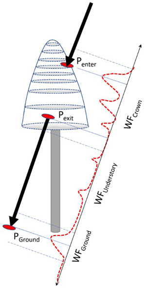
Fig. 8. Illustration of the capture of WF segments of a pulse that intersects the crown of a reference tree. Points Penter, Pexit and PGround are 3D intersection points used for splitting the entire WF between the segments. Because of convolution, the segments include amplitude values ‘before and after’ the ‘exact’ points and the segments have some overlap following Pexit and 1−2 m above the ground. WF attributes derived for the amplitude sequences are listed in Table 2.
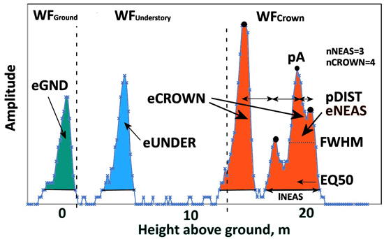
Fig. 9. An ALS60 WF of a 21.5-m-high pine. Graph illustrates the three WF segments and their WF attributes. WFCrown extends from 21 to 12 m and has four peaks (nCROWN = 4). eCROWN (crown energy) is the sum of amplitude values in WFCrown. pDist is the average distance between the peaks in WFCrown. The first-return NEAS amplitude sequence has three peaks (nNEAS = 3) and the length was 27 nanoseconds (lNEAS). The value of EQ50 is <0.5 as the NEAS energy is concentrated in the initial part. Understory energy (eUNDER) is due to the pulse intersecting the trunk or a dead branch 3−4 m above the ground. The pulse gave rise to a weak ground signal, and eGND (ground energy) is the sum of amplitude values belonging to WFGround. Echo width (FWHM) is computed using pA, which is the maximum amplitude in the NEAS.
2.6 Computation of WF attributes
Table 2 list the attributes that we computed for each pulse that intersected a crown and Fig. 9 illustrates them. We adopted many attributes by Hovi et al. (2016), who used several ALS60 datasets with 7.8−10.5-ns-long pulses. Because the return WFs of Q680i (4.5-ns-long pulses) showed much more details compared to ALS60, we extended the attribute list to include the split into the crown, understory and ground segments. Hovi et al. (2016) searched the ALS60 WFs for so-called first-return noise-exceeding amplitude sequences (NEAS), which in ALS60 data are fewer compared to Q680i. In order to maintain comparability to Hovi et al. (2016), we also implemented the NEAS approach. We, however, did not classify the pulses according to the discrete return information (first-of-many, single echo pulses etc.). Attributes MinRelDist, pADist, pARelDist and SZA were mainly included for control purposes. For example, pADist indirectly measures crown diameter and cannot be used for predicting tree species, but it was a useful variable for verifying the correctness of the algorithms. Similarly, the average SZA (scan zenith angle) was assumed to be affected by local tree height as shorter trees are occluded at high angles of SZA. It was not used as a predictor of tree species, although it might be useful in separating shade-tolerant species from light-demanding species in dense mixed stands.
| Table 2. WF attributes of each pulse intersecting a tree crown. Attributes marked with * were directly adopted from Hovi et al. (2016). See Fig. 8 for the definition of WF segments representing the crown, understory and ground. | |
| Attribute | Definition |
| eCROWN | Crown energy. Sum of amplitude values assigned to WFCrown |
| eNEAS* | Energy of the (first-return) noise-exceeding amplitude sequence, NEAS |
| eUNDER | Understory energy. Sum of amplitude values assigned to WFUnderstory |
| eGND | Ground energy. Sum of amplitude values assigned to WFGround |
| nCROWN | Number of local maxima in WFCrown |
| nNEAS* | Number of local maxima in the (first) NEAS |
| pA* | Maximum amplitude in the NEAS, ‘peak amplitude’ |
| FWHM* | Width of the echo giving pA, nanoseconds |
| lNEAS* | Total length of the NEAS, nanoseconds |
| pDist | Mean distance between local peaks in WFCrown, meters |
| MinRelDist | Minimum relative horizontal pulse-trunk distance inside the crown, 0−1 |
| pADist | Horizontal distance to the trunk of point pA, meters |
| pARelDist | Horizontal distance to the trunk of point pA, relative, 0−1 |
| EQ50 | Relative distance of the energy median from the start of the NEAS, 0−1 |
| SZA | Scan zenith angle, degrees |
2.7 Tree-level WF features
We computed the mean and standard deviation features of the WF attributes for each tree with more than four pulses intersecting the crown. Prefixes m_, and s_ denote the mean and standard deviation, respectively. Suffixes _1064 and _1550 denote the wavelength. For example, m_FWHM_1064 is the mean of the echo width attribute in ALS60 (1064 nm) pulses.
2.8 Statistical methods and analyses tools
We computed the arithmetic mean and standard deviation of the WF features by species class and applied correlation analyses to study the dependencies between the features as well as the correlation between the features and tree height. We used the F-test (lm and ANOVA-functions in R version 4.1.2) and the Gini-importance metric of the Random Forest (RF) algorithm (randomForest package in R (Liaw and Wiener 2002)) to assess feature importance for species classification, which was carried out using quadratic discriminant analyses (QDA) (MASS package in R (Venables and Ripley 2002)). Classification performance was measured using overall accuracy (OA, %) and the simple kappa (κ) metrics.
We programmed tools for WF processing, image interpretation and the photogrammetric tasks using C, Java, Visual basic and Excel VBA. WF attribute extraction was repeated using redundant Matlab code to minimize the chance of implementation errors.
3 Results
3.1 Differences of 1064 and 1550 nm features by species
Table 3 shows a comparison of all mean features by species normalized with respect to pine. Fig. 10 has separate box plot graphs for the eCROWN, lNEAS and FWHM mean features. Crown energy that is least affected by pulse length showed interspecies differences, especially in 1064 nm. Strikingly, dead spruce showed the lowest crown energy in 1064 nm, while it was the ‘brightest’ species class in 1550 nm. Alder had the highest eCROWN_1064 nm. Return energy from the understory was high in both living and dead spruces. In spruce, the crown ratio of 40% underestimates the true crown ratio and explains this observation in part. The length of the first-return NEAS (lNEAS) did not separate pine from spruce in 1064 nm but displayed discriminating power in 1550-nm data (Fig. 10). This is likely due to the better range resolution of the 1550 nm sensor. The high reflectance of spruce bark and wood influenced lNEAS_1550 such that dead spruce is not similarly separable as it is in lNEAS_1064. FWHM (echo width) measures target ‘softness’ and does not display distinct interspecies differences. Spruce and dead spruce showed the lowest values and represented ‘hard’ vegetation types among the tested species. Wavelength did not affect the relative order of m_FWHM by species.
| Table 3. Comparison of mean features by species relative to pine. Features are described in Table 2 and Fig. 9. The colors highlight the differences. Dead S refers to dead spruce. | |||||||
| Mean feature | Pine | Spruce | Birch | Aspen | Alder | Larch | Dead S |
| m_eCROWN_1064 | 100 | 120 | 136 | 140 | 165 | 135 | 86 |
| m_eUNDER_1064 | 100 | 151 | 138 | 135 | 105 | 127 | 135 |
| m_eGND_1064 | 100 | 60 | 64 | 40 | 44 | 66 | 136 |
| m_nCROWN_1064 | 100 | 103 | 108 | 109 | 104 | 106 | 117 |
| m_eNEAS_1064 | 100 | 118 | 135 | 139 | 166 | 135 | 79 |
| m_pA_1064 | 100 | 124 | 128 | 133 | 164 | 127 | 84 |
| m_nNEAS_1064 | 100 | 100 | 106 | 105 | 101 | 105 | 103 |
| m_lNEAS_1064 | 100 | 100 | 114 | 115 | 118 | 114 | 88 |
| m_FWHM_1064 | 100 | 93 | 104 | 101 | 98 | 104 | 94 |
| m_pDist_1064 | 100 | 107 | 109 | 114 | 121 | 102 | 108 |
| m_EQ50_1064 | 100 | 103 | 100 | 97 | 93 | 101 | 106 |
| m_MinRelDist_1064 | 100 | 101 | 104 | 105 | 103 | 102 | 95 |
| m_pARelDist_1064 | 100 | 93 | 103 | 106 | 112 | 104 | 90 |
| m_eCROWN_1550 | 100 | 95 | 105 | 82 | 111 | 115 | 146 |
| m_eUNDER_1550 | 100 | 125 | 106 | 102 | 95 | 119 | 198 |
| m_eGND_1550 | 100 | 86 | 88 | 68 | 80 | 86 | 114 |
| m_nCROWN_1550 | 100 | 97 | 105 | 110 | 114 | 103 | 100 |
| m_eNEAS_1550 | 100 | 92 | 105 | 77 | 109 | 115 | 142 |
| m_pA_1550 | 100 | 102 | 99 | 79 | 105 | 112 | 140 |
| m_nNEAS_1550 | 100 | 93 | 103 | 96 | 107 | 104 | 100 |
| m_lNEAS_1550 | 100 | 88 | 106 | 90 | 107 | 108 | 103 |
| m_FWHM_1550 | 100 | 96 | 104 | 106 | 106 | 105 | 98 |
| m_pDist_1550 | 100 | 99 | 105 | 109 | 110 | 99 | 101 |
| m_EQ50_1550 | 100 | 106 | 100 | 103 | 97 | 100 | 107 |
| m_MinRelDist_1550 | 100 | 98 | 103 | 106 | 105 | 102 | 85 |
| m_pARelDist_1550 | 100 | 92 | 103 | 107 | 111 | 105 | 78 |
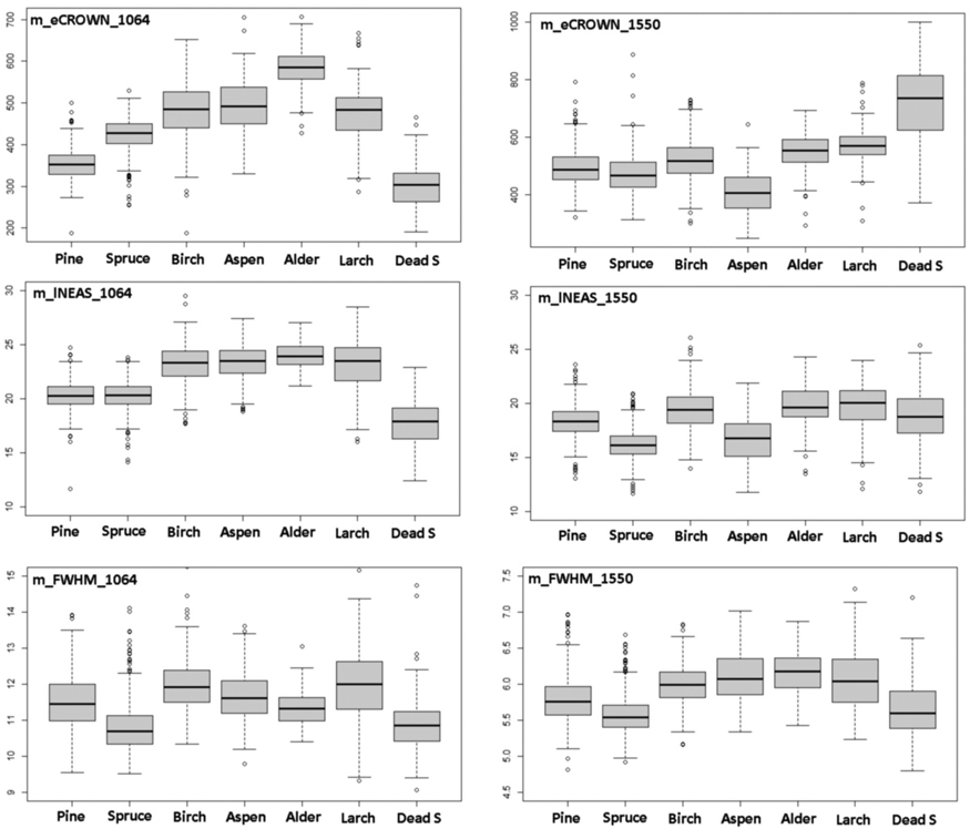
Fig. 10. Comparison of 1064-nm and 1550-nm features m_eCROWN, m_lNEAS and m_FWHM by species. Features are described in Table 2 and Fig. 9. View larger in new window/tab.
The number of peaks (nCROWN and nNEAS) showed moderate between-species variation, as did the average distance between WF peaks (pDist). Feature MinRelDist showed the lowest values for dead spruce, which is logical as their crowns comprise of dead branches, and the pulses can penetrate the envelope that is defined by the branch tips. The values were low also in living spruce, which makes sense given the branching pattern. The relative distance from the stem of the strongest echoes (pARelDist) showed the lowest values in spruce and dead spruce. Ground energy (eGND) of pulses that intersect the crowns displays an interesting and logical pattern. The eGND is high in dead spruces because less energy is absorbed in the crowns, and probably also because the bottom flora has changed (more reflective herb-vegetation owing to increased light) in areas with dead spruces. EQ50 measures the shape (‘center of gravity’) of the NEAS, and dead spruce shows the largest values suggesting that the return pulses (NEAS) have a slower rise.
3.2 Feature correlation with tree height
In Hyytiälä, the height of dominant trees correlates positively with stand age owing to the thin-from-below thinning rule, and thus, the results concerning height apply to age as well. Also, the site type variation that drives height growth was rather limited in our data. The reference trees represented dominant and intermediate canopy layers, as suppressed trees in closed canopies were not discernible in LiDAR. We can therefore consider that 10−15-m-high trees represented 25−40-year-old trees, and trees taller than 27−30 m were from 100−150-year-old stands. Table 4 shows the Pearson correlation coefficients between WF features and tree height. The number of WF peaks and their average distance (nCROWN, pDIST) correlated positively with tree height, which is logical as the crowns of tall trees are longer. Crown energy of both wavelengths (eCROWN) correlates positively with height in pine, spruce, and dead spruce, while in birch, the correlation was negative. Old larch had sparse foliage and showed lower 1064 nm crown energy compared to younger trees, while the opposite is true for 1550 nm. The bark of larch is highly reflective at 1550 nm, and its silhouette was probably more visible in old larches. Echo width (FWHM) is shorter in old conifers compared to young trees. The shoots of old conifers are ‘packed’ as the height growth has terminated. EQ50 correlated negatively with height in coniferous trees, suggesting that the shape of the returns changes with height/age.
| Table 4. Correlation of mean waveform features with tree height by wavelength (1064, 1550) and species. Features are described in Table 2 and Fig. 9. The colors highlight the differences. Dead S refers to dead spruce. | ||||||||||||||||
| 1064 | 1550 | 1064 | 1550 | 1064 | 1550 | 1064 | 1550 | 1064 | 1550 | 1064 | 1550 | 1064 | 1550 | 1064 | 1550 | |
| All | Pine | Spruce | Birch | Aspen | Alder | Larch | Dead S | |||||||||
| m_eCROWN | 0.01 | 0.30 | 0.40 | 0.66 | 0.36 | 0.53 | –0.22 | –0.23 | 0.01 | 0.17 | 0.10 | 0.06 | –0.44 | 0.21 | 0.30 | 0.42 |
| s_eCROWN | –0.01 | 0.23 | 0.34 | 0.63 | –0.04 | 0.33 | –0.15 | –0.20 | 0.19 | 0.17 | 0.15 | 0.16 | –0.14 | 0.42 | –0.21 | 0.12 |
| m_eUNDER | –0.07 | 0.07 | 0.14 | 0.22 | 0.04 | 0.13 | –0.29 | –0.18 | –0.23 | –0.36 | –0.14 | 0.14 | –0.29 | –0.19 | 0.17 | 0.24 |
| s_eUNDER | 0.02 | 0.14 | 0.16 | 0.23 | 0.27 | 0.29 | –0.23 | –0.06 | –0.09 | –0.12 | –0.18 | –0.13 | –0.25 | –0.16 | 0.25 | 0.28 |
| m_eGND | –0.22 | –0.06 | –0.36 | –0.20 | –0.41 | –0.11 | –0.28 | –0.13 | 0.00 | 0.04 | –0.57 | –0.51 | 0.13 | 0.30 | –0.59 | –0.33 |
| s_eGND | –0.10 | –0.05 | –0.27 | –0.05 | –0.16 | –0.18 | –0.11 | 0.04 | 0.18 | 0.02 | –0.50 | –0.30 | 0.18 | 0.23 | –0.48 | –0.24 |
| m_nCROWN | 0.39 | 0.50 | 0.18 | 0.31 | 0.51 | 0.70 | 0.40 | 0.44 | 0.23 | 0.62 | 0.26 | 0.40 | 0.45 | 0.65 | 0.52 | 0.56 |
| s_nCROWN | 0.44 | 0.60 | 0.21 | 0.51 | 0.57 | 0.72 | 0.48 | 0.56 | 0.39 | 0.70 | 0.31 | 0.50 | 0.41 | 0.66 | 0.48 | 0.63 |
| m_eNEAS | –0.05 | 0.17 | 0.31 | 0.55 | 0.17 | 0.31 | –0.27 | –0.36 | –0.03 | 0.04 | 0.04 | –0.09 | –0.47 | –0.11 | 0.20 | 0.23 |
| s_eNEAS | 0.09 | 0.25 | 0.43 | 0.63 | 0.27 | 0.41 | –0.08 | –0.25 | 0.24 | 0.09 | 0.21 | 0.08 | –0.07 | 0.47 | 0.05 | 0.22 |
| m_pA | 0.00 | 0.26 | 0.48 | 0.63 | 0.29 | 0.44 | –0.24 | –0.26 | 0.00 | 0.04 | 0.03 | –0.11 | –0.30 | 0.17 | 0.15 | 0.19 |
| s_pA | 0.11 | 0.29 | 0.44 | 0.54 | 0.45 | 0.55 | –0.03 | –0.06 | 0.18 | 0.09 | 0.07 | –0.12 | –0.16 | 0.30 | 0.05 | 0.15 |
| m_nNEAS | 0.05 | 0.11 | –0.22 | –0.25 | 0.07 | 0.26 | 0.11 | –0.09 | –0.08 | 0.14 | 0.04 | 0.10 | 0.01 | 0.02 | 0.30 | 0.42 |
| s_nNEAS | 0.11 | 0.23 | –0.19 | –0.12 | 0.16 | 0.33 | 0.18 | 0.07 | 0.06 | 0.23 | 0.05 | 0.23 | 0.07 | 0.28 | 0.32 | 0.49 |
| m_lNEAS | –0.05 | 0.02 | –0.24 | –0.27 | 0.01 | 0.08 | –0.07 | –0.24 | –0.02 | 0.08 | 0.08 | –0.04 | –0.44 | –0.29 | 0.30 | 0.34 |
| s_lNEAS | 0.15 | 0.26 | –0.10 | –0.09 | 0.16 | 0.37 | 0.20 | 0.01 | 0.23 | 0.28 | 0.24 | 0.29 | 0.24 | 0.54 | 0.29 | 0.43 |
| m_FWHM | –0.24 | –0.23 | –0.50 | –0.44 | –0.43 | –0.40 | –0.18 | –0.10 | –0.20 | –0.06 | –0.06 | –0.30 | –0.44 | –0.51 | 0.08 | –0.25 |
| s_FWHM | –0.01 | –0.16 | –0.11 | –0.34 | –0.07 | –0.21 | 0.03 | –0.05 | 0.08 | –0.13 | –0.12 | –0.15 | 0.00 | –0.45 | 0.02 | –0.09 |
| m_pDist | 0.50 | 0.55 | 0.61 | 0.71 | 0.63 | 0.63 | 0.55 | 0.63 | 0.46 | 0.62 | 0.42 | 0.41 | 0.48 | 0.69 | 0.28 | 0.31 |
| s_pDist | 0.52 | 0.50 | 0.58 | 0.63 | 0.61 | 0.58 | 0.51 | 0.51 | 0.41 | 0.51 | 0.32 | 0.32 | 0.46 | 0.49 | 0.35 | 0.24 |
| m_EQ50 | –0.24 | –0.21 | –0.43 | –0.42 | –0.32 | –0.31 | –0.35 | –0.12 | –0.29 | –0.20 | –0.15 | 0.06 | –0.35 | –0.06 | 0.03 | –0.17 |
| s_EQ50 | –0.09 | 0.00 | –0.08 | 0.05 | –0.10 | 0.00 | –0.05 | –0.01 | –0.23 | –0.03 | –0.12 | –0.09 | –0.18 | 0.11 | 0.25 | 0.11 |
| m_MinRelDist | –0.07 | –0.14 | –0.25 | –0.33 | –0.02 | –0.15 | –0.07 | –0.05 | 0.02 | –0.13 | –0.09 | –0.24 | –0.23 | –0.31 | 0.22 | 0.09 |
| s_MinRelDist | 0.07 | 0.12 | 0.08 | 0.16 | 0.11 | 0.21 | 0.01 | 0.23 | –0.11 | –0.21 | –0.50 | –0.07 | –0.09 | –0.05 | 0.14 | 0.12 |
| m_pARelDist | 0.30 | 0.23 | 0.36 | 0.33 | 0.37 | 0.31 | 0.48 | 0.45 | 0.26 | 0.27 | 0.01 | 0.16 | 0.25 | 0.34 | 0.32 | 0.23 |
| s_pARelDist | –0.14 | –0.08 | –0.27 | –0.13 | –0.30 | –0.15 | 0.06 | 0.11 | –0.16 | –0.25 | –0.12 | –0.06 | –0.03 | –0.10 | –0.29 | –0.07 |
3.3 Between-feature correlation
Fig. 11 shows the positive correlation of m_eCROWN and m_pARelDist features between the two wavelengths. Fig. 12 displays the entire correlation matrix. All diagonal values are positive i.e. the same 1064, and 1550-nm features were positively correlated. We could observe the strongest between-wavelength correlations for eGND, nCROWN, nNEAS, lNEAS, mFWHM, pDIST, EQ50 and the relative distance features. These are all ‘geometric features’ except for eGND (ground energy), which, however, is highly affected by crown energy losses. Feature m_EQ50_1064 showed a negative correlation with many of the 1550-nm features, but we could not explain why for example, the shape of the 1064-nm return pulse is in negative correlation with the mean relative distance of pulses giving rise to the 1550-nm peak signal (pARelDist). The interpretation is that a soft/delayed rise of the return WF is more likely in trees where the pulses penetrate the crown and reflect from near the stem.
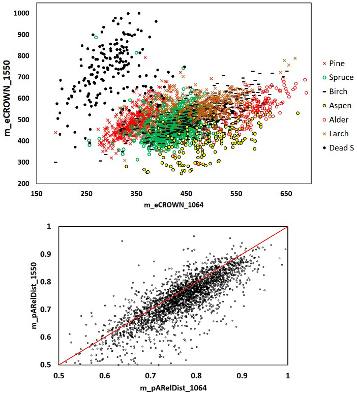
Fig. 11. 1064 and 1550 nm mean crown energy and mean relative distance of the strongest return from the trunk in 2532 trees. Dead spruce separates well in eCROWN_1064 and eCROWN_1550. Some of the outliers may be due to species errors in the field data or in image interpretation. The asymmetry of the m_pARelDist point pattern shows how the strongest echoes of 1550-nm pulses (36 cm footprint diameter) have reflected from farther off the stem compared to 1064-nm pulses (16 cm). Features are described in Table 2 and Fig. 9.
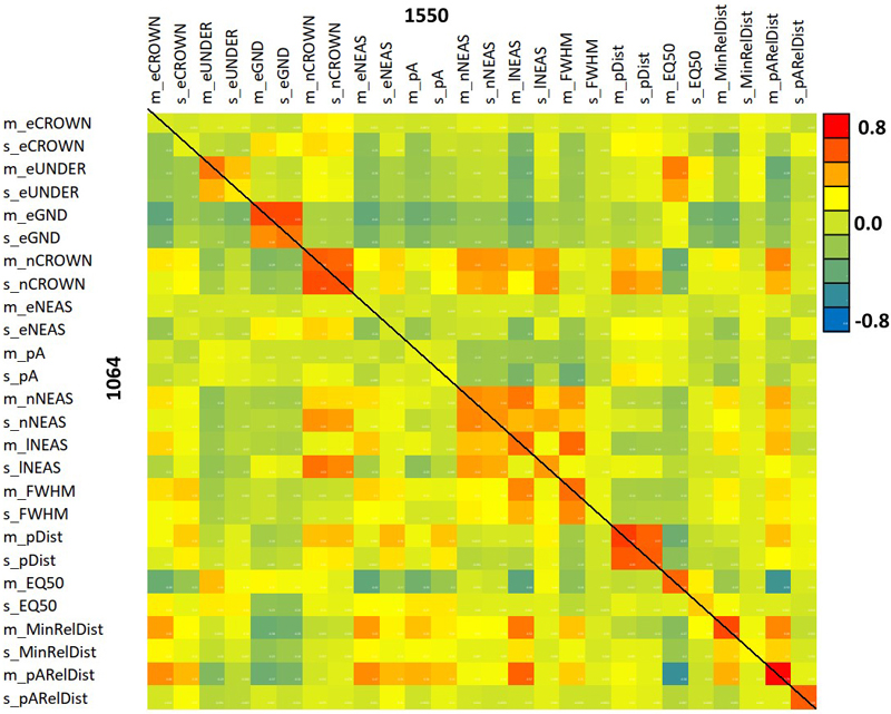
Fig. 12. Correlation between 1064 and 1550 nm features. The diagonal elements show the between-wavelength correlation of the same feature. Features are described in Table 2 and Fig. 9.
Fig. 13 shows the feature correlations separately for the two wavelengths. The patterns match only partially. For example, the negative correlation of 1064 nm features m_eGND and m_eCROWN is not observed in 1550 nm data. The correlation structure of both MinRElDist and pARelDist (see also Fig. 11) with other features shows between-band differences that we assume to relate to footprint diameter, which was 36 cm and 16 cm in the 1064 and 1550 nm data, respectively.
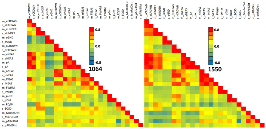
Fig. 13. Correlation of 1064 and 1550 nm features in all trees. Features are described in Table 2 and Fig. 9. View larger in new window/tab.
3.4 Species classification trials
We used rankings by F-test and the Gini-importance to select the predictors for the QDA classification. The total number of predictors was always ten. We classified first the full set of seven classes: pine, spruce, birch, dead spruce, aspen, alder and larch. Successive tests had fewer species by shortening the list from the end. We used repeated random subsampling validation such that 0, 10, 20, 50 or 80% of the data were randomly selected for validation, while 100, 90, 80, 50 or 20% of trees were used for estimating the QDA-model. These samples were generated 1000 times in each classification trial and the results were averaged. Table 5 shows the classification results. OA and kappa metrics improved in all trials when 1064 and 1550 nm data were fused. The reduction of the training data decreased accuracy, but the effect was not very strong to indicate model overfitting. Features selected by Gini-importance presented better performance compared to variables selected using the F-test. Slightly better accuracy was observed for 1550 nm compared to 1064 nm when the species list had more than 4 entries, but 1064 nm outperformed the 1550 nm data for the three main tree species – pine, spruce and birch. A high OA of almost 94% was attained in trials encompassing three or four species and dual-wavelength data. Table 6 shows an error matrix for the classification of seven species using dual-wavelength data. The accuracy of birch was the lowest and birch was confused with larch. Pine and dead spruce were classified most accurately (90%). The average classification accuracies by species classes when using 1064 nm data, 1550 nm data and their combination are shown in Table 7. The combination improved the identification of birch, aspen and alder in particular. The best predictors by F-test and Gini-importance metric that were used in the classifications are listed in Table 8. We can note that for example m_eCROWN was a discriminating feature in 1064 nm but less important in 1550 nm.
| Table 5. Average overall accuracy (OA,%) and kappa in QDA classifications using repeated (n = 1000) random sub-sampling validation with random splits between training and validation data using ratios 100:100, 90:10, 80:20, 50:50 and 20:80. Case 100:100 was computed only once and represents an optimistic scenario. Classification was done using 7, 6, 4 and 3 species classes using ten WF features ranked by F-test or Gini-importance. Only the range is given for kappa, not the values of all five validation scenarios. | |||||
| Classes | Wavelength | OA % with F-test variables | OA (%) with Gini-variables | F-test | Gini-vars |
| 100 90 80 50 20% | 100 90 80 50 20% | kappa | kappa | ||
| All seven | 1064 | 76.7 73.5 73.3 72.5 69.9 | 76.7 73.6 73.3 72.5 69.8 | 0.711→0.624 | 0.711→0.624 |
| 1550 | 78.1 76.0 75.9 75.6 73.3 | 80.3 78.1 77.9 77.5 75.1 | 0.729→0.669 | 0.756→0.691 | |
| 1064+1550 | 84.1 83.0 82.7 82.3 79.9 | 86.5 84.7 84.6 84.0 81.5 | 0.802→0.750 | 0.833→0.801 | |
| 6 classes, without larch | 1064 | 83.5 80.9 80.6 80.1 77.6 | 83.5 80.8 80.7 80.1 77.6 | 0.785→0.706 | 0.785→0.706 |
| 1550 | 83.2 81.6 81.6 81.0 79.1 | 84.0 82.3 82.4 81.7 79.5 | 0.783→0.727 | 0.793→0.732 | |
| 1064+1550 | 88.7 87.9 87.8 87.4 85.5 | 91.3 90.0 90.1 89.7 87.6 | 0.855→0.810 | 0.889→0.838 | |
| 4 classes, pine, spruce, birch, dead spruce | 1064 | 88.7 87.6 87.6 87.3 86.1 | 88.7 87.7 87.7 87.4 86.1 | 0.838→0.800 | 0.838→0.800 |
| 1550 | 88.2 87.3 87.2 86.8 85.7 | 89.0 88.1 88.1 87.8 86.7 | 0.831→0.795 | 0.842→0.809 | |
| 1064+1550 | 91.1 90.6 90.6 90.4 89.6 | 93.5 92.7 92.7 92.6 91.8 | 0.871→0.850 | 0.906→0.881 | |
| 3 classes, pine, spruce, birch | 1064 | 90.8 89.8 89.7 89.5 88.4 | 90.8 89.9 89.8 89.5 88.4 | 0.855→0.819 | 0.855→0.817 |
| 1550 | 88.7 87.9 87.6 87.1 85.9 | 89.2 88.4 88.4 88.0 86.8 | 0.824→0.780 | 0.830→0.793 | |
| 1064+1550 | 91.6 91.2 91.1 90.8 89.9 | 93.9 93.5 93.3 93.0 92.2 | 0.868→0.841 | 0.905→0.878 | |
| Table 6. Average confusion matrix in 1000 randomized validations using 80% of the trees for training and 20% for validation. The predictors were the five best 1064 and 1550 nm features by Gini-importance (Kappa = 0.808, OA = 84.6%). Dead refers to dead spruce. | |||||||
| QDA class | True class | ||||||
| Pine | Spruce | Birch | Aspen | Alder | Larch | Dead | |
| Pine | 436 | 19 | 9 | 10 | 4 | ||
| Spruce | 38 | 741 | 15 | 2 | 47 | 6 | |
| Birch | 4 | 13 | 328 | 23 | 13 | 60 | 1 |
| Aspen | 1 | 12 | 129 | 9 | 3 | ||
| Alder | 10 | 10 | 125 | 1 | |||
| Larch | 7 | 13 | 44 | 3 | 241 | ||
| Dead | 7 | 11 | 2 | 175 | |||
| Table 7. Average Producer’s accuracy (%) by species in classifications of seven species classes using predictors selected by Gini-importance (90:10 ratio of training and validation). Dead refers to dead spruce. | |||||||
| Wavelenght | Pine | Spruce | Birch | Aspen | Alder | Larch | Dead |
| 1064 nm | 87 | 85 | 51 | 46 | 78 | 61 | 79 |
| 1550 nm | 78 | 88 | 68 | 67 | 58 | 76 | 90 |
| 1064+1550 nm | 91 | 87 | 75 | 84 | 86 | 79 | 89 |
| Table 8. Feature ranking by F-test and Gini-importance in data combining all seven species. 1064 and 1550 refer to the wavelength. Features are described in Table 2 and Fig. 9. | |||
| F-test 1064 | F-test 1550 | Gini 1064 | Gini 1550 |
| m_eCROWN | s_eNEAS | m_lNEAS | m_lNEAS |
| m_eNEAS | s_eCROWN | m_eCROWN | s_pA |
| m_pA | m_eCROWN | s_pA | s_eNEAS |
| s_pA | m_eNEAS | m_eNEAS | m_pDist* |
| s_eNEAS | s_eUNDER* | m_pA | m_FWHM |
| m_lNEAS | m_pARelDist | m_FWHM | s_eCROWN |
| s_eCROWN | s_pA | s_eNEAS | m_eNEAS |
| m_pARelDist | m_eUNDER* | s_eCROWN | m_EQ50* |
| m_EQ50 | m_lNEAS | m_EQ50 | m_pARelDist |
| m_FWHM | m_pA* | m_pARelDist | m_eCROWN |
4 Discussion
4.1 Originality
We implemented a novel 3D capture of amplitude sequences that represent backscattering from crown, understory and the ground and combined it with the existing (first-return) NEAS attribute definitions by Hovi et al. (2016). We are unaware of studies that have combined airborne two-wavelength WF LiDAR data in tree species classification, so our results provide new insights. The use of airborne LiDAR WF features in the classification of aspen, dead spruce, alder, and larch is also unique, as previous studies in Scandinavia have focused on pine, spruce and birch.
4.2 Confines
Our experimental study had some limitations. The single-band sensors differed in properties that influenced the return signal (Table 1). Most notably, the length of the transmitted pulse (7.6 and 4.5 ns) and the at-target footprint diameter (36 and 16 cm) deviated between the datasets. Because of the shorter pulse length, LMS-Q680i data displayed more peaks in return WFs (nNEAS, nCROWN) with a smaller average distance and echo width (pDist, FWHM). Table 3 shows that relative to pine, the species-specific mean values of FWHM display rather similar patterns except for aspen and alder. However, footprint size influences the WFs and canopy transmission losses, as narrow pulses are more likely to ‘find gaps’ that are larger than the footprint, as shown by Korpela (2017). He compared WFs of ALS60 pulses with 11, 22, 44 and 59 cm diameter and showed that, compared to wider pulses, narrow pulses produce 17−38-% lower FWHM and 15−25-% higher pA and slightly (5−8%) lower eNEAS. There were also between-species differences in the responses. This also implies that wavelength was only one of many parameters that influenced our findings.
The acquisition of the 1550-nm LiDAR data took place early in the summer and the results concerning aspen may include minor phenological effects because aspens had just reached full-leaf state and were well the full-leaf state during the 1064-nm acquisition. The investigated trees represent dominant, co-dominant and intermediate trees that were discernible in LiDAR and could be estimated a parametric crown model, which was a circular-symmetric surface of revolution (Fig. 7). We used the models to assign pulses to individual trees using 3D ray intersection, but it is obvious that there were errors in this linking caused e.g. by crown asymmetry, small geometric noise of the pulses, individual long branches and close neighbors. Our manual 3D crown delineation likely outperforms automatic tree detection and delineation, which, however, are needed in real applications (Lindberg et al. 2014).
The number of species classes was high for a study conducted in Finland, but the number of reference trees was limited to 146−848 per class. We combined downy and silver birch into one class. Separation of the two would be beneficial for forest management, but it is considered highly ill-posed by means of airborne remote sensing because the morphological differences are so small. Trees younger than 25−30 years were missing entirely, and we only had 40-year-old alders. Our assumption of a 40% crown ratio was a compromise (Figs. 8, 9), and the WFUnder segments in living spruce included lower parts of the living crowns. Unfortunately, there were too few dead-standing pine or birch trees in the area, and we could only study dead spruce. Of species that may reach the dominant layer, we did not include goat willow (Salix caprea L.) and grey alder (Alnus incana (L.) Moench) because of their rarity.
There were parameters that influenced the computation of WF attributes, which we did not discuss in detail. For example, there were sensor-specific minimum length criteria for a plausible NEAS, and the peak amplitude of a NEAS had to reach a certain minimum (see also Hovi et al. 2016). The limit on pA in the LMS-Q680i data was influenced by ‘ringing’, which is present in the WFs and means that a strong echo is followed by a false weak peak following an 11 ns delay (Korpela et al. 2020). The peak shows dimly in Fig. 1. In ALS60, the WFs displayed low noise, and contrary to LMS-Q680i, in which the return WFs could consist of 1−3 sequences (lengths of 80, 160, 240) with pauses in between, the stored WFs of ALS60 were always 256-ns-long contiguous sequences, which is beneficial for the detection of weak backscattering in the canopy (Korpela et al. 2013). On the other hand, the fixed 256 ns length limits the use of ALS60 WFs to canopies lower than 35 m in height. We also applied modest low-pass filtering of the WFs. The filtering removed implausible adjacent peaks and small peaks caused by noise.
Our LiDAR data was collected from a height of 700−750 m, which means that acquisition costs were relatively high. It remains unknown if modern sensors can be operated from a higher altitude without major performance loss in signal-to-noise ratio or pulse density. Having several acquisition heights would have been beneficial but was out of reach because of excessive costs.
Sensors that we used are no longer in commercial use, and more efficient sensors have replaced them. Modern sensors, such as the VQ-series of scanners by Riegl and the Leica TerrainMapper-2, are based on online waveform processing but can store and output WFs according to product specifications. The storage of WFs can slow down the sensor (pulse repetition frequency), which decreases efficiency. It seems that fewer modern sensors utilize the 1550 nm wavelength, as 532 nm and 1064 nm seem to be preferred. The physics of the pulse-target convolution has not changed since our data was collected in 2013, but the sensors have. However, there is typically an interdependence (trade-off) between the radiometric and geometric traits of optical sensors and advances in the other may lead to worsened characteristics of the other properties. For example, the new single-photon LiDAR sensors can be flown at high altitudes, but the intensity data are noisy and have a low radiometric resolution. If the end-user only needs the coordinates of the first returns, this is not an issue, but if the intensity or WF data are essential, the low resolution may influence the results considerably.
4.3 Feature analyses
4.3.1 Correlation of WF features with tree size
Our results showed clearly that tree size (age, height growth rate) influenced the WF features, and that the direction of the relationships differed between species and even between wavelengths in some cases. Regarding ALS60 (1064 nm) and findings concerning pine, spruce and birch, our results are in line with those by Hovi et al. (2016). For example, crown energy diminished in old birches, which is likely due to lower leaf density of the large old crowns. An opposite positive correlation was observed in conifers, in which the mean crown energy increased with tree size. In larch, the trend differed between wavelengths as old larch trees gave rise to stronger returns on 1550 nm, while old larches were ‘darker’ in 1064 nm. The very high reflectance of larch bark at 1550 nm (Rautiainen et al. 2018) likely explains this and we can also note here that larch has shown by far the strongest returns among all Hyytiälä trees in leaf-off 1550-nm data captured in November 2011. In old larches, the foliage is sparse and more bark is exposed to the illuminating pulse. A negative correlation of echo width with tree size was the strongest in conifers and was observed in both sensors. We explain the ‘hardening of echoes’ by the shoot structure of old trees that have ceased to grow in height. This finding was also reported by Hovi et al. (2016) for pine and spruce.
4.3.2 Correlation of the 1064 and 1550 nm features
We observed that the same features were in a positive correlation between the 1064 and 1550 nm wavelengths. Features that measure crown geometry showed the strongest correlation, while radiometric features (energy, peak amplitude) displayed a weaker positive correlation. Feature m_pARelDist correlated strongly between wavelengths. It is the mean relative (trunk branch tip) distance of the strongest echoes. The correlation here measured a ‘tree effect’ (Hovi et al. 2016), and, in the case of m_pARelDist, the high correlation implies that the relative size order of trees was preserved between the first and second LiDAR acquisition that were separated by three weeks only. As noted earlier, the length of the transmitted pulse differed between the sensors, which likely weakened the correlations of other geometric features.
We did not observe any major influence by the scan zenith angle on any of the mean features (results not reported). For example, pARelDist was in a negative correlation with SZA in living and dead spruce, which implies that echoes of oblique pulses penetrated deeper into the crowns, which is logical.
4.3.3 Features by species classes
The ALS60 data that we used here was one of the four (2010−2013) ALS60 campaigns that were analyzed for living pine, spruce and birch by Hovi et al. (2016). Comparison of pA, eNEAS, FWHM and EQ50 mean features by species between the studies shows strong agreement, which was also observed in the correlation of WF features with tree size. The similarity of findings confirms in part that our algorithms for WF attribute computations were implemented correctly, and the trees in different parts of Hyytiälä share a similar structure (we used different reference trees). Hovi et al. (2016) reported that eNEAS_1064 constitutes a strong predictor in species classification, which we also could conclude for both eNEAS_1064 and eCROWN_1064, which correlate strongly in the ALS60 data owing to the long pulse length. Korpela (2017) has shown that eNEAS is also rather invariant to footprint size, which is a beneficial trait for a predictor variable.
Regarding the differences between 1064 and 1550 nm mean features, we could observe some important differences (Fig. 10, Table 3) that contributed towards improved classification results when combining the two bands. For example, dead spruce constituted ‘darkest objects’ in 1064 nm but displayed the largest mean eCROWN and pA in 1550 nm data. In spruce, the eCROWN was higher compared to pine in 1064 nm, but the opposite was true in 1550 nm.
4.3.4 Notes on dead standing spruces
Our results concerning WF features of dead spruce apply to trees that had died 1−10 years prior to the LiDAR campaign in 2013. By analyzing a time-series of high-resolution aerial images, we could note that some of them were dead already in 2004. It is evident that the structure of dead trees changes with time as branches and shoots fall on the ground. We have strong indication of this in LiDAR data that were acquired in 2011 and 2015 with the same 1550-nm sensor and acquisition settings that we used here (2013 data). We did not include the results here to limit the scope of this report, but the morphological changes of dead spruces over time increase within-class feature variation in this ‘species’ class. Thus, if the classification of dead spruces is done in an area, where the spruces have died within a short timeframe, the within-class feature variance will not be as large as we had, and an even higher classification performance (for dead spruce) can be expected.
4.4 Species classification
Our results suggest that combining 1064 and 1550-nm WF features improves the classification performance of pine, spruce, birch, alder, aspen, larch and dead spruce. We observed an overall accuracy (OA) of almost 87% for the seven classes, and it was 91% when the larch was removed. The OA was almost 94% when the classification was done between pine, spruce, birch and dead spruce. A part of the observed performance gain was due to the increase of pulses intersecting the crowns (random errors of features that showed positive correlation cancel out) when the datasets were fused. The gain was 3−10 percentage points being the highest when all seven species were classified. The use of 1550-nm WF features resulted in somewhat better classification accuracy compared to 1064 nm, when there were 6 or 7 classes, while the 1064-nm data was more accurate in the classification of pine, spruce and birch. However, this can also be partly caused by the more detailed WFs of the 1550-nm sensor. Crown energy (e_CROWN) at 1064 nm was an important predictor, which was also observed by Hovi et al. (2016) for the separation of pine, spruce, and birch.
Our results suggest that 1064-nm and 1550-nm WF features do not separate accurately birch from larch. However, larch is a relatively rare exotic species and typically forms single species stands. Dead spruce was classified with an accuracy of better than 90%, and they separated well in eCROWN_1064 and eCROWN_1550. Alder gives rise to strong returns in 1064 nm, which was observed by Korpela et. al. (2010) using discrete-return (Leica ALS50-ii sensor) intensity data, which is in high correlation with pA in Leica ALS50/60 series of receivers. Aspen was confused with birch and alder, and the accuracy remained at 85%. Our samples of aspen were dominant trees that were well discernible in the aerial images, and a lower level of accuracy may well be expected in dense canopies, where the crowns are smaller with fewer pulses per tree.
The QDA classifications were done using ten predictors (ten best single-band features and 5+5 when combining the datasets). We did also run the RF algorithm, and the OOB (out-of-the-box) error estimates did not deviate substantially from the QDA estimates.
5 Conclusions and suggestions for future work
Merging 1064 nm and 1550 WF features results in significantly improved classification performance compared to the use of a single wavelength in 30−150-year-old trees. However, even with dual-wavelength data, Siberian larch does not separate well from birch and Norway spruce. Aspen, which is an ecologically important species was confused with the other broadleaved species, birch and alder. Dead spruce creates a distinct class in dual-wavelength data, although we must note that the crowns of dead trees change as time passes, and this should be explored further. Because the length of the transmitted pulse and the footprint size differed between the two sensors, we cannot draw unambiguous conclusions about the superiority of particular features. However, we confirm the importance of 1064-nm crown energy that was shown by Hovi et al. (2016). If a choice should be made between the two wavelengths, we recommend 1064 nm for the main tree species in Finland. Sampling and storing of WF data often slow down the LiDAR sensor and results in vast amounts of data, but previous research clearly shows the benefits of single wavelength WF data (Reitberger et al. 2008; Hollaus et al. 2009; Heinzel and Koch 2011; Vaughn et al. 2012; Yu et al. 2014; Lindberg et al. 2014), and here we disclosed that combining 1064 and 1550-nm WFs creates a viable option for tree species classification. Our approach can most likely be improved by adding geometric (height-distribution) metrics that we omitted. If crown base height (CBH) estimation in LiDAR data is feasible (Vauhkonen 2010), WF segments representing the crown and the understory can be split more accurately, and CBH as such, constitutes a strong discriminating feature, especially between pine and spruce (Holmgren and Persson 2004). Single-tree remote sensing does not reach the suppressed trees, but we suggest research in the use of understory WF segments to see if they contain any species information about the occluded trees. In addition, the use of both leaf-off and leaf-on WF data is an unexplored option and may well enhance the classification accuracy of deciduous trees that vary in branching pattern and leaf-orientation.
Declaration of openness of research materials, data, and code
Binary LiDAR data, source code and tree measurements are available from the corresponding author upon request.
Authors’ contributions
IK conceived the research idea and wrote most of the code and measured the crown models. All authors took part in the statistical analyses, searched the literature and participated in writing and commenting on the manuscript in Finnish. AP wrote parallel Matlab code for WF processing to minimize the chance of implementation errors. IK wrote the English version, which was revised by AP.
Acknowledgements
This study was conducted on course FOR-254 ‘Advanced Forest Inventory and Management Project’ at the University of Helsinki. Plots IM and OG were measured by students and assistants on course FOR110B with the kind permission of Prof. Pauline Stenberg. Dr. Pekka Kaitaniemi provided phenological observations during LiDAR campaigns, and support by Dr. Antti Uotila was crucial in finding aspen, alder and larch samples in Hyytiälä.
Funding
The LiDAR and field data in 2013 were collected and processed with funding from the Academy of Finland and Metsämiesten säätiö. Other work by made possible by the University of Helsinki.
References
Ahokas E, Kaasalainen S, Hyyppä J, Suomalainen J (2006) Calibration of the Optech ALTM3100 laser scanner intensity data using brightness targets. Rev Française Photogramm Télédet 182: 10−16. https://www.isprs.org/proceedings/XXXVI/part1/Papers/T03-11.pdf.
Anderson K, Hancock S, Disney M, Gaston KJ (2016) Is waveform worth it? A comparison of LiDAR approaches for vegetation and landscape characterization. Remote Sens Ecol Conserv 2: 5−15. https://doi.org/10.1002/rse2.8.
Blomley R, Hovi A, Weinmann M, Hinz S, Korpela I, Jutzi B (2017) Tree species classification using within crown localization of waveform LiDAR attributes. ISPRS J Photogramm Remote Sens 133: 142−156. https://doi.org/10.1016/j.isprsjprs.2017.08.013.
Danson M, Sasse F, Schofield LA (2018) Spectral and spatial information from a novel dual-wavelength full-waveform terrestrial laser scanner for forest ecology. Interface Focus 8, article id 20170049. https://doi.org/10.1098/rsfs.2017.0049.
Disney MI, Kalogirou V, Lewis P, Prieto-Blanco A, Hancock S, Pfeifer M (2010) Simulating the impact of discrete-return lidar system and survey characteristics over young conifer and broadleaf forests. Remote Sens Env 114: 1546−1560. https://doi.org/10.1016/j.rse.2010.02.009.
Fassnacht FE, Latifi H, Stereńczak K, Modzelewska A, Lefsky M, Waser LT, Starub C, Ghosh A (2016). Review of studies on tree species classification from remotely sensed data. Remote Sens Env 186: 64−87. https://doi.org/10.1016/j.rse.2016.08.013.
Hancock S, Armston J, Li Z, Gaulton R, Lewis P, Disney M, Danson M, Strahler A, Schaaf C, Anderson K, Gaston K (2015) Waveform lidar over vegetation: an evaluation of inversion methods for estimating return energy. Remote Sens Env 164: 208–224. https://doi.org/10.1016/j.rse.2015.04.013.
Heinzel J, Koch B (2011) Exploring full-waveform LiDAR parameters for tree species classification. Int J Appl Earth Obs and Geoinf 13: 152–160. https://doi.org/10.1016/j.jag.2010.09.010.
Hollaus M, Mücke W, Höfle B, Dorigo W, Pfeifer N, Wagner W, Bauerhansl C, Regner B (2009) Tree species classification based on full-waveform airborne laser scanning data. Silvilaser, College Station, Texas, USA.
Holmgren J, Persson Å (2004) Identifying species of individual trees using airborne laser scanner. Remote Sens Env 90: 415–423. https://doi.org/10.1016/S0034-4257(03)00140-8.
Holmgren J, Persson Å, Söderman U (2008) Species identification of individual trees by combining high resolution LiDAR data with multi-spectral images. Int J Remote Sens 29: 1537–1552. https://doi.org/10.1080/01431160701736471.
Hovi A (2015) Towards an enhanced understanding of airborne LiDAR measurements of forest vegetation. Diss For 200. Finnish Society of Forest Research. https://doi.org/10.14214/df.200.
Hovi A, Korpela I (2013) Real and simulated waveform-recording LiDAR data in juvenile boreal forest vegetation. Rem Sens Env 140: 665–678. https://doi.org/10.1016/j.rse.2013.10.003.
Hovi A, Korhonen L, Vauhkonen J, Korpela I (2016). LiDAR waveform features for tree species classification and their sensitivity to tree- and acquisition related parameters. Remote Sens Env 173: 224–237. https://doi.org/10.1016/j.rse.2015.08.019.
Hu T, Sun X, Su Y, Guan H, Sun Q, Kelly M, Guo Q (2020) Development and performance evaluation of a very low-cost UAV-Lidar system for forestry applications. Remote Sensing 13, article id 77. https://doi.org/10.3390/rs13010077.
Korpela I (2006) Geometrically accurate time series of archived aerial images and airborne lidar data in a forest environment. Silva Fenn 40: 109–126. https://doi.org/10.14214/sf.355.
Korpela I (2017) Acquisition and evaluation of radiometrically comparable multi-footprint airborne LiDAR data for forest remote sensing. Remote Sens Env 194: 414–423. https://doi.org/10.1016/j.rse.2016.10.052.
Korpela I, Tuomola T, Välimäki E (2007) Mapping Forest plots: an efficient method combining photogrammetry and field triangulation. Silva Fenn 41: 457–469. https://doi.org/10.14214/sf.283.
Korpela I, Tokola T, Orka HO, Koskinen M (2009) Small-footprint discrete-return lidar in tree species recognition. In: Proceedings of the ISPRS Hannover Workshop 2009, Hannover, Germany, 2–5 June 2009, pp 1–6.
Korpela I, Ørka HO, Maltamo M, Tokola T, Hyyppä J (2010) Tree species classification using airborne LiDAR – effects of stand and tree parameters, downsizing of training set, intensity normalization and sensor type. Silva Fenn 44: 319–339. https://doi.org/10.14214/sf.156.
Korpela I, Heikkinen V, Honkavaara E, Rohrbach F, Tokola T (2011) Variation and directional anisotropy of reflectance at the crown scale – implications for tree species classification in digital aerial images. Remote Sens Env 115: 2062–2074. https://doi.org/10.1016/j.rse.2011.04.008.
Korpela I, Hovi A, Korhonen L (2013) Backscattering of individual LiDAR pulses explained by photogrammetrically derived vegetation structure. ISPRS J Photogramm Remote Sens 83: 81–93. https://doi.org/10.1016/j.isprsjprs.2013.06.002.
Korpela I, Haapanen R, Korrensalo A, Tuittila ES, Vesala T (2020) Fine-resolution mapping of microforms on a boreal bog using aerial images and waveform-recording LiDAR. Mires and Peat 26, article id 03. https://doi.org/10.19189/MaP.2018.OMB.388.
Koukal T, Atzberger C (2012) Potential of multi-angular data derived from a digital aerial frame camera for forest classification. IEEE J Sel Topics in Appl Earth Obs and Remote Sens 5: 30–43. https://doi.org/10.1109/JSTARS.2012.2184527.
Kukkonen M, Maltamo M, Korhonen L, Packalén P (2019) Multispectral airborne LiDAR data in the prediction of boreal tree species composition. IEEE Trans Geosci Remote Sens 57: 3462–3471. https://doi.org/10.1109/TGRS.2018.2885057.
Liaw A, Wiener M (2002) Classification and regression by randomForest. R News 2: 18–22.
Lim K, Treitz P, Wulder M, St-Onge B, Flood M (2003) LiDAR remote sensing of forest structure. Progress Physical Geog 27: 88–106. https://doi.org/10.1191/0309133303pp360ra.
Lindberg E, Eysn L, Hollaus M, Holmgren J, Pfeifer N (2014) Delineation of tree crowns and tree species classification from full-waveform airborne laser scanning data using 3-D ellipsoidal clustering. IEEE J Sel Topics Appl Earth Obs and Remote Sens 7: 3174–3181. https://doi.org/10.1109/JSTARS.2014.2331276.
Mallet C, Bretar F (2009) Full-waveform topographic lidar: state-of-the-art. ISPRS J Photogramm Remote Sens 64: 1−16. https://doi.org/10.1016/j.isprsjprs.2008.09.007.
Maltamo M, Packalén P (2014) Species-specific management inventory in Finland. In: Maltamo M, Næsset E, Vauhkonen J (eds) Forestry applications of airborne laser scanning: concepts and case studies. Managing Forest Ecosystems 27, Springer, pp 241–252. https://doi.org/10.1007/978-94-017-8663-8_12.
Mäyrä J, Keski-Saari S, Kivinen S, Tanhuanpää T, Hurskainen P, Kullberg P, Poikolainen L, Viinikka A, Tuominen S, Kumpula T, Vihervaara P (2021) Tree species classification from airborne hyperspectral and LiDAR data using 3D convolutional neural networks. Remote Sens Env 256, article id 112322. https://doi.org/10.1016/j.rse.2021.112322.
Pisek J, Chen J, Miller J, Freemantle J, Peltoniemi J, Anita S (2010) Mapping forest background reflectance in a boreal region using multiangle compact airborne spectrographic imager data. IEEE Transact Geosci Remote Sens 48: 499–510. https://doi.org/10.1109/TGRS.2009.2024756.
Rana P, St-Onge B, Prieur JF, Brindusa C, Tolvanen A, Tokola T (2022) Effect of feature standardization on reducing the requirements of field samples for individual tree species classification using ALS data. ISPRS J Photogramm Remote Sens 184: 189–202. https://doi.org/10.1016/j.isprsjprs.2022.01.003.
Rautiainen M, Lukeš P, Homolová L, Hovi A, Pisek J, Mõttus M (2018) Spectral properties of coniferous forests: a review of in situ and laboratory measurements. Remote Sens 10, article id 207. https://doi.org/10.3390/rs10020207.
Reitberger J, Krzystek P, Stilla U (2008) Analysis of full waveform LIDAR data for the classification of deciduous and coniferous trees. Int J Remote Sens 29: 1407−1431. https://doi.org/10.1080/01431160701736448.
Roncat A, Briese C, Jansa J, Pfeifer N (2014) Radiometrically calibrated features of full-waveform lidar point clouds based on statistical moments. IEEE Geosci Remote Sens Lett 11: 549−553. https://doi.org/10.1109/LGRS.2013.2274557.
Swatantran A, Tang H, Barrett T, DeCola P, Dubayah R (2016) Rapid, high-resolution forest structure and terrain mapping over large areas using single photon lidar. Sci Rep 6, article id 28277. https://doi.org/10.1038/srep28277.
Ullrich A, Pfennigbauer M (2011) Echo digitization and waveform analysis in airborne and terrestrial laser scanning. In: Fritsch D (ed) Photogrammetric week ’11: 217−228. Stuttgart, Germany, September 5−9. https://ifpwww.ifp.uni-stuttgart.de/publications/phowo11/220Ullrich.pdf.
Vaughn NR, Moskal LM, Turnblom EC (2012) Tree species detection accuracies using discrete point lidar and airborne waveform lidar. Remote Sens 4: 377−403. https://doi.org/10.3390/rs4020377.
Vauhkonen J (2010) Estimating crown base height for Scots pine by means of the 3D geometry of airborne laser scanning data. Int J Remote Sens 31: 1213−1226. https://doi.org/10.1080/01431160903380615.
Vauhkonen J, Maltamo M, McRoberts RE, Næsset E (2014). Introduction to forestry applications of airborne laser scanning. In: Maltamo M, Næsset E, Vauhkonen J (eds) Forestry applications of airborne laser scanning: concepts and case studies. Springer, The Netherlands, pp 1–16. https://doi.org/10.1007/978-94-017-8663-8_1.
Venables WN & Ripley BD. (2002). Modern applied statistics with S, 4th edition. Springer, New York. ISBN 0-387-95457-0. https://www.stats.ox.ac.uk/pub/MASS4/.
Wagner W (2010) Radiometric calibration of small-footprint full-waveform airborne laser scanner measurements: basic physical concepts. ISPRS J Photogramm Remote Sens 65: 505−513. https://doi.org/10.1016/j.isprsjprs.2010.06.007.
Wagner W, Ullrich A, Ducic V, Melzer T, Studnicka, N (2006) Gaussian decomposition and calibration of a novel small-footprint full-waveform digitising airborne laser scanner. ISPRS J Photogramm Remote Sens 60: 100−112. https://doi.org/10.1016/j.isprsjprs.2005.12.001.
White J, Woods M, Krahn T, Papasodoro C, Bélanger D, Onafrychuk C, Sinclair I (2021) Evaluating the capacity of single photon lidar for terrain characterization under a range of forest conditions. Remote Sens Env 252, article id 112169. https://doi.org/10.1016/j.rse.2020.112169.
Yao W, Krzystek P, Heurich M (2012) Tree species classification and estimation of stem volume and DBH based on single tree extraction by exploiting airborne full-waveform LiDAR data. Remote Sens Env 123: 368−380. https://doi.org/10.1016/j.rse.2012.03.027.
Yu X, Litkey P, Hyyppä J, Holopainen M, Vastaranta M (2014) Assessment of low density full-waveform airborne laser scanning for individual tree detection and tree species classification. Forests 5: 1011−1031. https://doi.org/10.3390/f5051011.
Total of 47 references.
