Sakari Tuominen  ,
Reija Haapanen
,
Reija Haapanen
Estimation of forest biomass by means of genetic algorithm-based optimization of airborne laser scanning and digital aerial photograph features
Tuominen S., Haapanen R. (2013). Estimation of forest biomass by means of genetic algorithm-based optimization of airborne laser scanning and digital aerial photograph features. Silva Fennica vol. 47 no. 1 article id 902. https://doi.org/10.14214/sf.902
Abstract
Information on forest biomass is required for several purposes, including estimation of forest bioenergy resources and forest carbon stocks. Airborne laser scanning is today considered the most accurate remote sensing method for forest inventory. The three-dimensional nature of laser scanning data enables estimation of the volumes of the tree canopies. The dimensions of the tree canopies show high correlation with the amount of forest biomass. Optical aerial photographs are often used to complement laser data, for improved distinction between tree species. The paper reports on a study testing the estimation of forest biomass variables in two study areas in Southern Finland. The biomass variables were derived on the basis of tree-level field measurements, with biomass models used for pine, spruce, and birch. The sample-plot-level biomass components were derived on the basis of tree-level data and used as reference data for airborne-laser- and aerial‑photograph-based estimation. Results were slightly better for total biomass (RMSE 22.5% and 23.6% for the two study areas) than total volume (RMSE: 23.4% and 26.1%). Species-specific estimation errors were large in general but varied between the study areas, because of differences in their forest structures.
Keywords
forest inventory;
airborne laser scanning;
biomass modelling
-
Tuominen,
Finnish Forest Research Institute, P.O.Box 18, FI-01301 Vantaa, Finland
E-mail
sakari.tuominen@metla.fi
- Haapanen, Finnish Forest Research Institute, P.O.Box 18, FI-01301 Vantaa, Finland E-mail reija.haapanen@gmail.com
Received 18 July 2012 Accepted 16 January 2013 Published 11 June 2013
Views 177255
Available at https://doi.org/10.14214/sf.902 | Download PDF

1 Introduction
Accurate estimates of forest biomass are required for several purposes. Demand for forest biomass for bioenergy consumption is increasing markedly, supported by, for example, requirements imposed by EU directives for promotion of the use of energy from renewable sources (e.g., Steierer 2010). Industrial bioenergy-users need up-to-date information in cartographic form on the location and quantity of forest biomass resources. Forests also have a key role in the carbon cycle, and forest biomass is a significant carbon sink. Estimates of forest carbon stocks and predictions of their change are required for implementation of effective climate policy.
For a long time, remote sensing and earth observation techniques have been applied to produce mapped estimates of forest parameters such as the volume of growing stock. Typical remote sensing data sources that have been utilised are optical satellite images and aerial photographs. A forest inventory technique based on satellite imagery has been applied for estimation of forest biomass as well (e.g., Tucker et al. 1983; Roy and Ravan 1996; Tuominen et al. 2010; Nichol and Sarker 2011). Variables related to the quantity of aboveground forest biomass are well suited to remote-sensing-based estimation, since the canopy reflectance is correlated with the entire volume of forest biomass. This also holds true for active remote sensing techniques, such as airborne laser scanning (ALS), wherein the laser pulses reflected from the forest crown layer are used in prediction of forest characteristics.
In Finland, a new generation forest inventory system has been introduced for forest management planning. The new-generation system replaces the traditional visual inventory by stand. Estimation of forest variables in this new-generation forest inventory method is based on interpretation of ALS data and digital aerial photographs, with application of field measurements from sample plots as reference data. Typical sources of remote sensing data used in the system are low-density ALS data (typically 0.5–2 pulses/m2) and digital aerial photographs with a spatial resolution of 0.25–0.5 m, typically including the following spectral channels: blue (B), green (G), red (R), and near-infrared (NIR).
In the new forest inventory method the inventory units are square shaped elements of a systematic grid (i.e. grid cells). For the selection of the field plots the inventory area is typically stratified on the basis of earlier stand inventory data, and the field plots are allocated into these strata in order to get representative reference data covering all major types of forest for the interpretation of forest variables.
Currently, ALS is considered to be the most suitable remote sensing method for estimation of stand-level forest variables (Næsset 2002; Næsset 2004; Maltamo et al. 2006). Compared with optical-remote-sensing data sources, ALS data are particularly well suited to estimation of forest attributes related to physical dimensions of tree canopies, because ALS produces three-dimensional (3D) information on forest canopies. On the other hand, ALS data are not as well suited to estimation of tree species proportions or dominance with the applied point density (e.g., Törmä 2000). Therefore, optical imagery usually is needed to complement the ALS data. Aerial photographs have been widely used in forest inventory and their affordability and availability are generally good (e.g., Tuominen and Pekkarinen 2005; Maltamo et al. 2006).
The combination of aerial photographs and ALS data makes it possible to derive a very large number of remote sensing features describing the characteristics of a field plot or a stand. Consequently, the dimensionality of the remote sensing feature space increases greatly. It is, in general, computationally infeasible to use all possible remote sensing features when processing large inventory areas. Also, when the dimensionality grows, the data become sparse in relation to the dimensions (Hinneburg et al. 2000). This causes problems for estimators based on distance or proximity in the feature space (‘the curse of dimensionality’; e.g., Beyer et al. 1999). Therefore, the number of remote sensing features must be reduced in a way that produces an appropriate subset of features for the estimation procedure, considering their usefulness in predicting the forest attributes as well as their mutual correlation. Many types of feature selection algorithms have been applied for this purpose (e.g., Siedlecki and Sklansky 1989; Pudil et al. 1994; Jain and Zongker 1997; Kudo and Sklansky 1998; Kudo and Sklansky 2000). In remote sensing-aided forest inventory applications e.g. correlation analysis (Tuominen and Pekkarinen 2005; Breidenbach et al. 2010), canonical analysis (Packalén et al. 2012), stepwise selection using various criteria and proceeding either forwards by adding or backwards by eliminating features, or combining these operations (Tuominen and Pekkarinen 2005; Maltamo et al. 2006; Packalén and Maltamo 2007; Haapanen and Tuominen 2008; Hudak et al. 2008; Packalén et al. 2009; Latifi et al. 2010; Breidenbach et al. 2010; Packalén et al. 2012), simulated annealing (Packalén et al. 2012) and genetic algorithms (e.g. Van Coillie et al. 2005; Haapanen and Tuominen 2008; Latifi et al. 2010) have been used.
The current plan of operation for the new-generation forest inventory system is to cover the area of the private forests of Finland in approximately 10 years with aerial photographs and ALS data. In the current inventory system, mainly growing stock variables related to stem dimensions and volume will be estimated. However, it would be relatively straightforward to also include variables related to forest biomass in the inventory system, by means of existing biomass modes. The estimation of forest biomass by means ALS and aerial imagery or other optical remote sensing data has been examined in several studies (e.g. Lefsky et al. 2005; van Aardt et al. 2006; Popescu 2007; Næsset and Gobakken. 2008; Kotamaa et al. 2010; Hauglin et al. 2012).
The objective of this study was to test ALS- and aerial-photograph-based estimation of forest biomass. We focus on feature selection, as it is an important aspect in cases where a multitude of potential image features is available. Two study areas were taken into analyses, because in earlier studies, we have seen differing estimation success of individual tree species depending on the forest composition of the study area. In addition, the most optimal set of features often differ between study areas.
2 Materials and methods
2.1 Study areas and field data
The laser-scanning- and aerial-image-based estimation was tested in two study areas. Study area 1 was in the municipality of Lammi, in Southern Finland (approximately 61°19´N, 25°11´E). The area covered approximately 1800 ha of state-owned forest. The field data employed in this study encompassed 263 fixed-radius (9.77 m) circular plots that were measured in 2007. From each plot, all living tally trees with a breast-height diameter of at least 50 mm were measured. The total number of trees measured in this study area was 8027. For each tally tree, the following variables were recorded: location, tree species, crown layer, diameter at breast height, height, and height of living crown. The plots were located with Trimble’s GEOXM 2005 Global Positioning System (GPS) device, and the locations were processed with local base station data, with an average error of approximately 0.6 m. The forests in the study area were dominated by coniferous tree species, mainly Scots pine (Pinus sylvestris) and Norway spruce (Picea abies). Of the deciduous species, birches (Betula pendula and B. pubescens) were most common. Other, mainly non-dominant tree species present in the study area were aspen (Populus tremula), grey alder (Alnus incana), rowan (Sorbus aucuparia), contorta pine (Pinus contorta), larches (Larix spp.), and firs (Abies spp.).
Study area 2 was located in Eastern Finland, in the municipalities of Kuopio and Karttula (approximately 62°55´N, 27°12´E), covering approximately 36 700 ha of mainly privately owned forest. The field data employed in this study covered 504 fixed-radius (9.00 m) sample plots measured in 2009. In each plot, all living tally trees with a breast-height diameter of at least 50 mm were measured. The total number of tally trees measured in this area was 14 657. The following variables were measured for each tally tree: species, crown layer, tree class, and diameter at breast height. Height and age were measured from sample trees used for each tree species and crown layer. The tally trees’ heights were estimated via a model by Eerikäinen (2009) developed for generalisation of sample trees’ characteristics to tally trees. The model is based on locally calibrated species-specific dependence between stem diameter and height. The field plots were located with a high-precision GPS device, and the locations were processed with local base station data. The accuracy of the field plot positioning was specified to be 1 m. The forests in the study area were dominated by coniferous tree species, and Norway spruce was the dominant tree species, with approximately half of the total volume, followed by Scots pine. The deciduous species, making up less than a quarter of the volume, were mainly birches (Betula pendula and B. pubescens). The proportion of other species was insignificant.
In order to cover all types of forest, the study areas were stratified on the basis of earlier stand inventory data and the field sample plots were assigned to these strata. The statistics of the study areas, from the sample plot measurements, are presented in Tables 1 and 2. In both areas, Scots pine and Norway spruce were treated as separate classes and other species as one class. In study area 1, this group then included a variety of species (‘other species’), but in study area 2 only deciduous species. The locations of the study areas and the field sample plot layouts within them are presented in Fig. 1. Fig. 2 shows the distribution of total aboveground (ABVG) biomass in both areas.
| Table 1. Forest statistics of study area 1 (average, maximum and standard deviation of values for the 263 sample plots used). | |||
| Forest variable | Average | Max. | Std. |
| Total stem volume, m3/ha | 190.9 | 575.4 | 109.1 |
| Stem volume of Scots pine, m3/ha | 74.5 | 560.6 | 87.8 |
| Stem volume of Norway spruce, m3/ha | 68.0 | 575.4 | 96.6 |
| Stem volume of other species, m3/ha | 48.4 | 312.0 | 56.7 |
| Total ABVG biomass, tonnes/ha | 96.4 | 251.8 | 50.4 |
| ABVG biomass of Scots pine, tonnes/ha | 34.2 | 197.3 | 38.2 |
| ABVG biomass of Norway spruce, tonnes/ha | 35.4 | 251.8 | 46.7 |
| ABVG biomass of other species, tonnes/ha | 26.7 | 164.3 | 30.2 |
| Total biomass of branches, tonnes/ha | 19.2 | 54.5 | 10.5 |
| Biomass of Scots pine branches, tonnes/ha | 5.7 | 36.7 | 6.2 |
| Biomass of Norway spruce branches, tonnes/ha | 9.3 | 54.4 | 11.3 |
| Biomass of other species’ branches, tonnes/ha | 4.1 | 27.9 | 4.5 |
| Table 2. Forest statistics for study area 2 (average, maximum, and standard deviation of values for the 504 sample plots used). | |||
| Forest variable | Average | Max. | Std. |
| Total stem volume, m3/ha | 206.5 | 798.5 | 126.3 |
| Stem volume of Scots pine, m3/ha | 51.8 | 577.6 | 81.7 |
| Stem volume of Norway spruce, m3/ha | 111.3 | 739.2 | 130.4 |
| Stem volume of deciduous species, m3/ha | 43.4 | 400.4 | 64.6 |
| Total ABVG biomass, tonnes/ha | 110.0 | 341.9 | 59.5 |
| ABVG biomass of Scots pine, tonnes/ha | 25.1 | 229.5 | 37.6 |
| ABVG biomass of Norway spruce, tonnes/ha | 60.5 | 325.1 | 66.0 |
| ABVG biomass of deciduous species, tonnes/ha | 24.3 | 214.9 | 35.7 |
| Total biomass of branches, tonnes/ha | 22.8 | 75.6 | 14.1 |
| Biomass of Scots pine branches, tonnes/ha | 4.8 | 36.0 | 6.8 |
| Biomass of Norway spruce branches, tonnes/ha | 16.2 | 75.5 | 16.4 |
| Biomass of deciduous species branches, tonnes/ha | 1.7 | 18.0 | 2.6 |
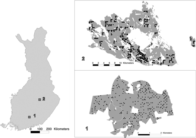
Fig. 1. The location of study areas 1 and 2 within Finland, and the spatial distribution of the field plots within the study areas.
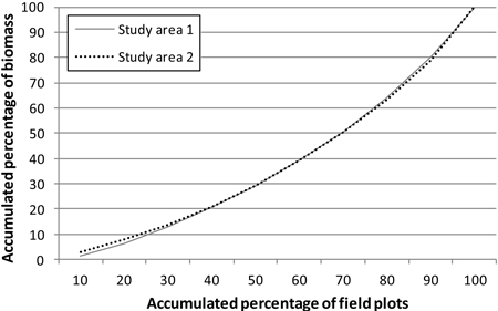
Fig. 2. Total aboveground biomass (per hectare) distribution in the study areas.
2.2 Remote sensing data
In study area 1, the remote sensing data consisted of orthorectified colour-infrared digital aerial photographs from 2006 (containing near-infrared, red, and green bands) with a ground resolution of 0.5 m and ALS data from 2006 acquired from a flying altitude of 1900 m with an average density of 0.88 pulses/m2. The aerial photographs were combined into an image mosaic covering the entire study area.
In study area 2, digital aerial photographs were acquired in 2008 from an altitude of 5600 m with an overlap of 60%. The images were orthorectified with 0.5 m ground resolution and featured blue, green, red, and near-infrared bands. ALS data were acquired in 2008, from a flying altitude of 2000 m. The density of the ALS data was 0.6 pulses/m.
In addition to the ALS point data, the ALS height and intensity data (of the first or only pulses) were interpolated to a raster format with a resolution similar to that of the aerial photographs. The output pixel values were calculated as inverse-distance-weighted (with a power of 2) averages of the two nearest ALS points. These raster images were used for computation of the textural features (see Subsection 2.4).
2.3 Estimation of biomass components
Sample-plot-level biomass quantities were estimated for the tally trees on the basis of the tree measurements. The main interest was in the total ABVG biomass; in addition, also branch and needle/foliage biomass was computed. Scots pine models were applied for all pines (Pinus sylvestris and P. contorta). Norway spruce models were applied for Norway spruce, larches, and firs (Picea abies, Larix spp., and Abies spp.). Birch models were applied for all deciduous tree species.
The following models were applied for estimation of biomass components in study area 1:
- Stem volume: volume models for Scots pine, Norway spruce, and birch by Laasasenaho (1982) utilising height and diameter as independent variables.
- Branch biomass: multivariate models for Scots pine and Norway spruce by Repola (2009) and multivariate model for birch by Repola (2008) based on diameter, height, and length of the living crown.
- Needle/foliage biomass: multivariate models for Scots pine and Norway spruce by Repola (2009) based on diameter, height, and length of the living crown and multivariate model for birch by Repola (2008) based on the diameter and crown ratio.
- Total ABVG biomass: multivariate models for Scots pine and Norway spruce by Repola (2009) based on diameter, height, and length of the living crown and multivariate model for birch by Repola (2008) based on diameter and height.
In study area 2, where the variable ‘length of the living crown’ was not measured in the field, the biomass estimation differed from that in study area 1 for a number of biomass components. The following models were applied in estimation of those biomass components in study area 2:
- Stem volume: volume models for Scots pine, Norway spruce, and birch by Laasasenaho (1982) utilising height and diameter as independent variables.
- Branch biomass: multivariate models for Scots pine and Norway spruce by Repola (2009) and multivariate model for birch by Repola (2008) based on diameter and height.
- Needle/foliage biomass: multivariate models for Scots pine and Norway spruce by Repola (2009) based on diameter and height, and multivariate model for birch by Repola (2008) based on diameter.
- Total ABVG biomass: multivariate models for Scots pine and Norway spruce by Repola (2009) based on diameter and height.
The sample-plot-level biomass quantities were calculated by summing of tree-level biomasses and conversion to tons per hectare.
2.4 Extraction of laser and aerial photograph features
A multitude of features can be derived from the registered ALS point altitudes, starting from the simplest ones, such as mean and maximum, which describe the stand height. Variables related to the range, deviation and distribution of point altitudes within the forest estimation units describe the canopy structure and they have been found suitable for area-based (i.e. stand level) estimation at the applied ALS point density (e.g. Naesset 2002; Naesset 2004). In applications using higher point densities and aiming at individual tree estimation also other features can be used, such as alpha shape metrics that describe the shape of individual canopies (e.g. Vauhkonen et al. 2012). Spectral averages and standard deviations of aerial photograph bands within the field plots vary according to canopy closure and tree species, although they are also dependent on other factors (such as sensor aperture and location in the image) that weaken the correlation (e.g. Tuominen and Pekkarinen 2004). Textural features of both remotely sensed data types describe the horizontal structure of the canopy, which, in turn, is affected by the tree species, canopy size and closure. The following statistical and textural features were extracted from the aerial photographs and ALS data for each sample plot area or from a square window centred on the sample plot:
- Averages and standard deviations of raster image pixel values of a 20 x 20 m window
- Standard deviations of raster image pixel values of blocks into which a 32 x 32 pixel window was divided. The blocks corresponded to 1 x 1, 2 x 2, 4 x 4, and 8 x 8 pixels. In addition to these four standard deviation values, the combined standard deviation of the blocks was computed (Wang et al. 1996).
- Textural features of raster images based on standard deviations and co-occurrence matrices of pixel values (Haralick et al. 1973; Haralick 1979) extracted for a 20 x 20 m window.
- Height distribution statistics of ALS point data for the first and last pulses extracted from the sample plot area. These included mean, standard deviation, maximum, coefficient of variation, heights at which certain percentages of points (5, 10, 20, ..., 95) had accumulated, and percentages of points accumulating at certain relative heights (5, 10, 20, ..., 95). Only points above 2 m were considered in the computation of these variables. Finally, the percentage of points over 2 m high was included as a variable.
In study area 1, also Normalized Difference Vegetation Index and near-infrared/red channel transformations were derived from the aerial photographs and features of sets 1–3 computed as above. This was expected to aid in the discrimination of biomass and volume by species. They were, however, rarely selected for the final feature sets in the feature selection procedure (see Subsection 2.5), so the process was not repeated for study area 2. Estimation with laser features only was tested in both areas as well.
For the estimation of forest biomass attributes, all features were standardised to a mean of 0and a standard deviation of 1. This was done because the original features had diverse scales of variation. Without standardisation, variables with wide variation would have greater weight in the estimation, regardless of their correlation with the estimated forest attributes, when using estimation methods that are based on proximity or distance in the feature space such as k-means clustering or k-nearest-neighbour method, which was applied in this study.
2.5 Estimation and feature selection methods
The k-nearest-neighbour (k-nn) method was used for estimating the forest variables (e.g., Kilkki and Päivinen 1987; Tomppo 1991; Tokola et al. 1996). In remote sensing based forest inventory applications the k-nn has distinct advantages compared to, e.g., regression modelling. In practical inventories the number of inventory variables is often high. In k-nn all inventory variables can be estimated simultaneously and k-nn is also likely to retain their original covariance structure of the inventory variables, whereas, when using regression analysis, the variables must be estimated separately or in groups, which may lead to estimates whose covariance structure is different from that of the original field variables, and not necessarily compatible estimates, in addition to a laborious estimation procedure (e.g. Tomppo and Halme 2004; Wilson et al. 2012).
In the k-nn method, Euclidean distances between the sample plots were calculated in the n-dimensional feature space, where n represents the number of features extracted. The estimates for the tested variables were calculated as weighted averages of the variables of the k nearest sample plots (Eq. 1). Weighting by inverse squared Euclidean distance in the feature space was applied (Eq. 2) to reduce the bias of the estimates (Altman 1992).
The value of k was set to 5, which is a compromise suitable for this kind of study not exploring the utility of the k-nn method as such.

where
ŷ = estimate for variable y
yi = measured value of variable y on the ith nearest neighbour plot

di = Euclidean distance (in the feature space) to the ith nearest neighbour plot
k = number of nearest neighbours
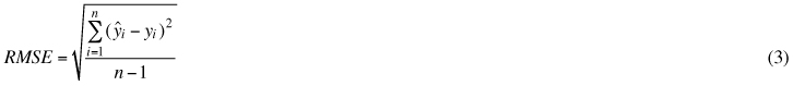
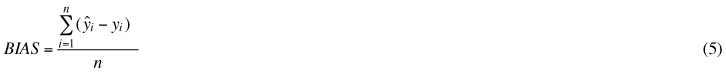
The estimated variables were total volume of growing stock; volumes of Scots pine, Norway spruce, and deciduous/other species; total ABVG biomass and biomasses, by species; and total biomass of branches + foliage and these biomasses, by species. Later in the text, the combined branch and foliage biomass is referred to as ‘branch biomass’. The accuracy of the estimates was calculated via leave-one-out cross-validation through comparison of the estimated forest variable values with the measured values (ground truth) of the field plots. The accuracy of the estimates was measured in terms of the relative root mean square error (RMSE) and bias (see Eqs. 3–6).
![]()
![]()
where
yi = measured value of variable y on plot i
ŷi = estimated value of variable y on plot i
y̅= mean of the observed values
n = number of plots
In order to select an appropriate set of features for the estimation task, automatic feature selection was carried out through a simple genetic algorithm (GA) presented by Goldberg (1989) and implemented in the GAlib C++ library (Wall 1996). The method has been successfully used for problems of similar types (e.g., Haapanen and Tuominen 2008; Tuominen and Haapanen 2011). The GA process starts by generating an initial population of strings (chromosomes or genomes), which consist of separate features (genes). The strings evolve over a user-defined number of iterations (generations). This evolution includes the following operations: selecting strings for mating by applying a user-defined objective criterion (the better, the more copies in the mating pool), allowing the strings in the mating pool to swap parts (cross over), causing random noise (mutations) in the offspring (children), and passing the resulting strings to the next generation. Here the starting population was 300 strings, which were developed over 30 generations. The probability of cross-over was 80% and that of a mutation one per cent. The objective was to minimise the RMSE of total biomass (or stem volume, depending on the case). When tree species biomasses or volumes were taken into account in the feature selection criteria, we created an artificial univariate response variable which was a weighted combination of species-specific relative RMSEs. The following weights were applied: total 55%, Scots pine 15%, Norway spruce 15%, deciduous/other species 15%. As the result depends on the randomly generated initial population, three 30-generation runs were completed. The expected proportion of activated features to all features is 50%, which means that with a large initial number of features, finding a good combination with only a few features is unlikely. Therefore, the features found in the best run were used as the base for a new selection step. In all, 3–4 of these GA steps were taken before the RMSEs stopped falling (see Fig. 3 in ‘Results’).
3 Results
3.1 The number and properties of the selected features
Features selected by the GA when both laser and aerial photograph features were available are listed in Appendix 1, and Table 3 summarizes the number of selected features in different cases. Fewer features were needed for the estimation of total amounts (biomass or volume) as compared with the situation wherein the success of species-specific estimation too was considered in the feature selection. In study area 2, there were more ALS features than aerial photograph features available for the first step of feature selection (52% of features), but in study area 1 the situation was the reverse (46% of the features were laser-based). After feature selection, ALS features dominated in both areas. Of the ALS feature types, those describing the vertical distribution of observations (bullet point 4 in section 2.4.) dominated. Some ALS intensity features were selected in most cases. The proportion of aerial photograph features was greater when species-specific RMSEs were employed in the GA. In study area 1, nearly all aerial photograph features selected were various textural features based on grey level co-occurrence matrices (Haralick et al. 1973). In study area 2, also spectral averages of grey values and various standard deviations were included in the optimised feature sets. It was expected that the number of features needed would be greater in the case in which only laser features were given as the starting population, but that was not the case – there was no clear pattern (see Table 4). In some cases, more Haralick textural features or standard deviation-based features (bullet points 2 and 3 in section 2.4) were selected when only ALS features were available, but no clear pattern could be detected there, either. However, total amounts again required fewer features than did species-specific amounts.
| Table 3. Number of features selected in each case when both laser and aerial photograph features were available. Percentage of aerial photograph features is in parentheses. | ||
| GA optimization case | Study area 1 | Study area 2 |
| Minimize RMSE of total volume | 12 (25%) | 18 (28%) |
| Minimize RMSE of total ABVG biomass | 9 (11%) | 8 (25%) |
| Minimize RMSE of total volume and species-specific volumes | 15 (47%) | 21 (33%) |
| Minimize RMSE of total ABVG biomass and species-specific ABVG biomasses | 13 (31%) | 17 (29%) |
| Table 4. Number of features selected in each case when only laser features were available. | ||
| GA optimization case | Study area 1 | Study area 2 |
| Minimize RMSE of total volume | 16 | 13 |
| Minimize RMSE of total ABVG biomass | 9 | 16 |
| Minimize RMSE of total volume and species-specific volumes | 16 | 15 |
| Minimize RMSE of total ABVG biomass and species-specific ABVG biomasses | 12 | 19 |
The effect of reducing the numtber of features step by step with the genetic algorithm is demonstrated in Fig. 3. The objective was to minimise the RMSE of total biomass of study area 1. The best feature combination found from among the three 30-generation repetitions was used as input for a new round of repetitions. At the starting point, all laser and aerial photograph features were available. The generation in which the lowest RMSE of the repetition was found varied between 5 and 29. The figure shows that during the consecutive steps:
- The RMSEs become generally lower
- The difference between the lowest RMSE of the first generation and the lowest RMSE found in the full course of the repetition diminishes
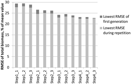
Fig. 3. Lowering of the RMSEs during the steps taken in the genetic algorithm process. The objective was to minimise the total ABVG biomass of study area 1. In each step, three 30‑generation repetitions are made, after which the best feature combination is used as the starting point for the next step.
3.2 Accuracies in the estimation of biomass and volume
Results were slightly better for total biomass than for total volume (see Tables 5 and 6). Species-specific estimation errors were large. In study area 1, the species had fairly even proportions in terms of the volumes and biomasses, which was reflected in the relatively uniform RMSE percentages. Taking the tree-species-specific estimates into account in the feature selection process reduced their error, but not much. Fig. 4 presents the residual biomasses (observed – estimated) in study area 1. Total biomasses have large errors in case of largest biomasses, whereas species-specific biomasses have large errors along the whole biomass distribution. In study area 2, the dominance of Norway spruce is noticeable in the clearly lower RMSE value among the species and the small effect of considering the species-specific errors in the feature selection. For Scots pine and other (deciduous) species, the residuals are large along the whole biomass distribution, as in study area 1 (Fig. 5). Branch biomass results were similar to total ABVG biomass results. In the case of Norway spruce, and in study area 2 also Scots pine, slightly lower relative RMSEs were obtained for branch biomass than for total ABVG biomass. Biases of total amounts were small in relation to the mean values. In study area 1, species-specific biases were also low, but in study area 2, volume of other species and biomasses of all species had some notable bias. When feature selection based solely on total amounts, the biases were generally larger than when taking into account the tree-species-specific estimates.
| Table 5. Relative stem volume RMSEs and biases (% of mean values) for study areas 1 and 2, where the forest variables used in the objective criterion in the feature selection process were total volume and volumes of Scots pine, Norway spruce, and other tree species (values obtained with minimisation of only the RMSE of total volume in the feature selection process are in brackets). | ||||
| Forest variable | Study area 1 | Study area 2 | ||
| RMSE | Bias | RMSE | Bias | |
| Total stem volume | 27.5 (23.4) | 0.7 (2.3) | 28.5 (26.1) | 0.4 (0.2) |
| Volume of Scots pine | 70.9 (98.3) | 0.2 (0.1) | 121.1 (128.9) | 0.5 (9.0) |
| Volume of Norway spruce | 78.8 (109.6) | 0.5 (6.8) | 57.6 (58.7) | 1.7 (6.6) |
| Volume of other species | 75.6 (101.0) | 2.4 (0.8) | 91.1 (96.9) | 6.9 (7.4) |
| Table 6. Relative ABVG biomass RMSEs and biases (% of mean values) for study areas 1 and 2, where both aerial photograph and laser features were used in the estimation and the forest variables used in the objective criterion in the feature selection process were total biomass and biomass figures for Scots pine, Norway spruce, and other tree species (values obtained with minimisation of only the RMSE of total biomass in the feature selection process are in brackets). | ||||
| Forest variable | Study area 1 | Study area 2 | ||
| RMSE | Bias | RMSE | Bias | |
| Total ABVG biomass | 24.8 (22.5) | 0.7 (1.3) | 24.5 (23.6) | 0.3 (0.5) |
| ABVG biomass of Scots pine | 66.9 (83.4) | 3.5 (4.7) | 109.9 (132.5) | 4.6 (5.2) |
| ABVG biomass of Norway spruce | 75.8 (95.3) | 2.0 (9.7) | 51.5 (55.4) | 6.7 (3.4) |
| ABVG biomass of other species | 75.7 (90.7) | 0.6 (2.1) | 92.6 (111.3) | 10.6 (6.1) |
| Total ABVG biomass of branches | 30.4 (30.1) | 0.1 (2.5) | 32.2 (34.6) | 3.4 (1.6) |
| ABVG biomass of Scots pine branches | 68.5 (84.2) | 2.9 (4.2) | 103.7 (124.4) | 4.2 (3.5) |
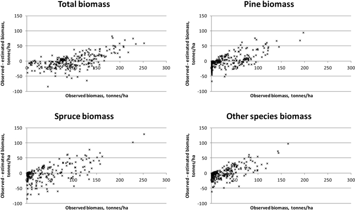
Fig. 4. Residuals of biomasses on study area 1. Species-specific biomasses were taken into account in the feature selection process.
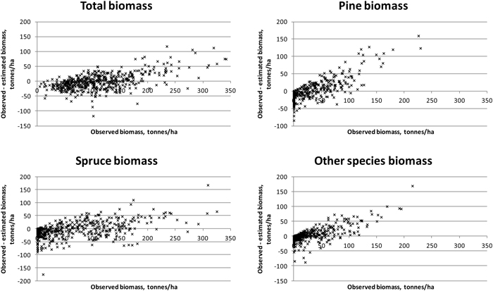
Fig. 5. Residuals of biomasses on study area 2. Species-specific biomasses were taken into account in the feature selection process.
In estimation with laser features only, slightly lower RMSEs were obtained for total ABVG biomass and total volume in study area 1 than with the use of both types of features. There the GA was not able to eliminate unnecessary aerial photograph features. In study area 2, combined feature sets produced lower RMSEs. In species-specific estimation, the aerial photograph features were useful in both areas (see Table 7).
| Table 7. Relative stem volume and ABVG biomass RMSEs and biases (% of mean values) for study areas 1 and 2. In this case, only laser features were used in the estimation and the forest variables used in the objective criteria in the feature selection process are total volume or biomass and volume (biomass) figures for Scots pine, Norway spruce, and other tree species (values obtained with minimisation of only the RMSE of total volume or biomass in the feature selection process are in brackets). | ||||
| Forest variable | Study area 1 | Study area 2 | ||
| RMSE | Bias | RMSE | Bias | |
| Total stem volume | 26.1 (22.9) | 1.1 (0.4) | 30.6 (28.5) | 0.7 (1.4) |
| Volume of Scots pine | 74.2 (88.8) | 5.3 (5.3) | 134.2 (139.3) | 6.9 (3.6) |
| Volume of Norway spruce | 83.5 (96.4) | 3.6 (4.7) | 61.9 (65.0) | 6.9 (8.5) |
| Volume of other species | 88.2 (96.3) | 1.2 (3.2) | 105.4 (119.3) | 6.2 (10.8) |
| Total ABVG biomass | 24.3 (22.1) | 0.7 (0.1) | 27.4 (24.8) | 1.3 (1.3) |
| ABVG biomass of Scots pine | 70.9 (91.2) | 3.7 (7.2) | 117.9 (133.5) | 8.0 (6.3) |
| ABVG biomass of Norway spruce | 74.7 (102.7) | 0.4 (4.3) | 61.8 (70.6) | 9.9 (9.8) |
4 Discussion
Airborne laser was found to be a suitable method for biomass estimation and can also be used without supporting aerial photography. The accuracy of the aboveground biomass estimates was on similar or slightly lower level than achieved by e.g. Kotamaa et al. (2010) in similar conditions, although in our study area 1 the number of field reference observations was lower, and in study area 2 the distribution of field variables was wider than in study material used by Kotamaa et al.
Concerning the nature of features selected for the estimation of biomasses or volumes, the following clear patterns were detected:
- The ALS-based features dominated the final feature combinations
- Fewer features were needed for the estimation of total amounts as compared with species-level estimation
- Aerial photograph features were always useful when species-level estimation accuracy was of interest
- Of the aerial photograph features, the Haralick textural features especially were selected.
Despite the benefit of having aerial photograph-based features available when estimating species-level biomasses or volumes, the results with ALS-based features only were not too far. Contrary to expectations, estimation with purely ALS-based features did not require a larger number of features, nor was the nature of selected ALS features different, compared with the cases when both remotely sensed data types were available.
For ABVG biomasses, lower relative RMSEs were obtained than for stem volumes. This seems to confirm the idea that laser features describe the canopy biomass better than they do the stem dimensions. It is noteworthy that we used stem volumes and biomasses obtained using models based on measurements of few tree variables. Furthermore, canopy width, a parameter appearing in more accurate biomass models, was not measured in the field in study area 2, and the height was measured from sample trees only, with the rest of the heights being based on modelling. One could ask: ‘Shouldn’t the results be more or less similar, as the same tree measurements were used both in biomass and in volume models?’ However, the biomasses and volumes are not completely linearly correlated on the stands, as different tree species and tree development stages have different biomasses in comparison with stem volumes (see Fig. 6). The unexplained variation of the biomass models that were applied in this study (Repola et al. 2007) is significantly higher than that seen under the volume models (Laasasenaho 1982). From Laasasenaho’s work (ibid.), the relative prediction error for Scots pine volume was 7–8%, whereas it was approximately 30–40% for, e.g., the foliage biomass (Repola et al. 2007). Some of the tally trees in both study areas considerably exceeded the diameter range of the sample trees used in the construction of the biomass models (Repola 2008; Repola 2009), but these account for a minor amount of the total tree mass (at approximately 100 trees in each study area).
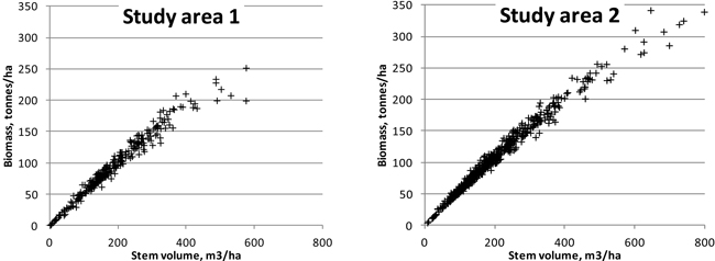
Fig. 6. Relationship of plot-level stem volumes with aboveground biomasses in the study areas.
In this study, we used biomass models that were published for the main tree species present in the study areas. In many cases, there are no models readily available for converting tree measurements to biomass weights, in which case it is necessary to harvest biomass samples from sample trees for laboratory analyses. If there is great variation in tree species, large samples covering different biomass fractions may be required for modelling forest biomass content (e.g., Nichol and Sarker 2011).
Despite the differences between the study areas, the relative estimation errors for total amounts of ABVG biomass and volume were very similar. Differences were observed in species-specific errors, where the errors were many times those seen for the total estimates. In both study areas, the dominant tree species showed the lowest estimation errors, as there is a larger number of suitable field plots in the nearest-neighbour estimation and thus finding a stand consisting of a ‘correct’ tree species is more likely. The relative error of the tree species biomass or volume was taken into account with a weight of 15% in the feature selection. Even with this low weight, a species obtaining very high relative RMSEs (typically a low percentage of the total volume) will probably have an unreasonably great impact on the features selected.
In this study, the estimations were carried out at the sample plot level. Another option would be the estimation of biomass components for individual trees. The individual-tree approach typically requires higher laser pulse density than this area-based approach does, making the inventory procedure more costly. Furthermore, even with a considerably higher pulse density, not all trees would be recognised by airborne sensor, because of tree canopies intermingling with each other or being hidden beneath larger trees.
5 Conclusions
The results of this study indicate that ALS in combination with aerial photography is well suited to the estimation of the variables related to the ABVG wood biomass. Since the same data are already in operational use for estimation of stem-related forest variables, the operational forest inventory could be similarly extended to ABVG biomass, through application of the same methodology. The resulting biomass maps should contribute greatly to the utilisation of forest biomass as a renewable energy source, as well as to the knowledge of forest carbon storage.
References
Altman N.S. (1992). An introduction to kernel and nearest-neighbor nonparametric regression. The American Statistician 46: 175–185.
Beyer K.S., Goldstein J., Ramakrishnan R., Shaft U. (1999). When is ‘nearest neighbor’ meaningful? Proceedings of the 7th International Conference on Database Theory (ICDT), Jerusalem, Israel, 10–12 January 1999. p. 217–235.
Breidenbach J., Næsset E., Lien V., Gobakken T., Solberg S. (2010). Prediction of species specific forest inventory attributes using a nonparametric semi-individual tree crown approach based on fused airborne laser scanning and multispectral data. Remote Sensing of Environment 114(4): 911–924.
Eerikäinen K. (2009). A multivariate linear mixed-effects model for the generalization of sample tree heights and crown ratios in the Finnish National Forest Inventory. Forest Science 55(6): 480–493.
Goldberg D.E. (1989). Genetic algorithms in search, optimization, and machine learning. Addison-Wesley Publishing Company, Reading, Massachusetts. 412 p.
Haapanen R., Tuominen S. (2008). Data combination and feature selection for multi-source forest inventory. Photogrammetric Engineering and Remote Sensing 74(7): 869–880.
Haralick R. (1979). Statistical and structural approaches to texture. Proceedings of the IEEE 67(5): 786–804.
Haralick R.M., Shanmugan K., Dinstein I. (1973). Textural features for image classification. IEEE Transactions on Systems, Man and Cybernetics SMC-3(6): 610–621.
Hinneburg A., Aggarwal C.C., Keim D.A. (2000). What is the nearest neighbor in high dimensional spaces? Proceedings of the 26th Very Large Data Bases (VLDB) Conference, 10–14 September 2000, Cairo, Egypt. p. 506–515.
Hauglin M., Gobakken T., Lien V., Bollandsas O.M., Næsset E. (2012). Estimating potential logging residues in a boreal forest by airborne laser scanning. Biomass and Bioenergy 36: 356–365
Hudak A.T., Crookston N.L., Evans J.S., Hall D.E., Falkowski M.J. (2008). Nearest neighbor imputation of species-level, plot-scale forest structure attributes from LiDAR data. Remote Sensing of Environment, 112(5): 2232–2245. Corrigendum: Remote Sensing of Environment 113(1): 289–290.
Jain A., Zongker D. (1997). Feature selection: evaluation, application, and small sample performance. IEEE Transactions on Pattern Analysis and Machine Intelligence 19: 153–157.
Kilkki P., Päivinen R. (1987). Reference sample plots to combine field measurements and satellite data in forest inventory. Department of Forest Mensuration and Management, University of Helsinki, Research Notes 19: 210–215.
Kotamaa E., Tokola T., Maltamo M., Packalén P., Kurttila M., Mäkinen A. (2010). Integration of remote sensing-based bioenergy inventory data and optimal bucking for stand-level decision making. European Journal of Forest Research 129: 875–886
Kudo M., Sklansky J. (1998). Classifier-independent feature selection for two-stage feature selection. Advances in pattern recognition. Lecture Notes in Computer Science 1451: 548–554.
Kudo M., Sklansky J. (2000). Comparison of algorithms that select features for pattern classifiers. Pattern Recognition 33: 25–41.
Laasasenaho J. (1982). Taper curve and volume functions for pine, spruce and birch. Communicationes Instituti Forestalis Fenniae 108.
Latifi H., Nothdurft A., Koch B. (2010). Non-parametric prediction and mapping of standing timber volume and biomass in a temperate forest: application of multiple optical/LiDAR-derived predictors. Forestry 83(4): 395–407.
Lefsky M.A., Turner D.P., Guzy M., Cohen W.B. (2005). Combining lidar estimates of aboveground biomass and Landsat estimates of stand age for spatially extensive validation of modelled forest productivity. Remote Sensing of Environment 95: 549–558
Maltamo M., Malinen J., Packalén P., Suvanto A., Kangas J. (2006). Nonparametric estimation of stem volume using airborne laser scanning, aerial photography, and stand-register data. Canadian Journal of Forest Research 36(2): 426–436.
Næsset E. (2002). Predicting forest stand characteristics with airborne scanning laser using a practical two-stage procedure and field data. Remote Sensing of Environment 80: 88–99.
Næsset E. (2004). Practical large-scale forest stand inventory using a small airborne scanning laser. Scandinavian Journal of Forest Research 19: 164–179.
Næsset E., Gobakken T. (2008). Estimation of above- and belowground biomass across regions of the boreal forest zone using airborne laser. Remote Sensing of Environment 112: 3079–3090.
Nichol J.E., Sarker M.L.R. (2011). Improved biomass estimation using the texture parameters of two high-resolution optical sensors. IEEE Transactions on Geoscience and Remote Sensing 49(3): 930–948.
Packalén P., Maltamo M. (2007). The k-MSN method for the prediction of species-specific stand attributes using airborne laser scanning and aerial photographs. Remote Sensing of Environment 109: 328–341.
Packalén P., Suvanto A., Maltamo M. (2009). A two stage method to estimate species specific growing stock by combining ALS data and aerial photographs of known orientation parameters. Photogrammetric Engineering and Remote Sensing 75(12): 1451–1460.
Packalén P., Temesgen H., Maltamo M. (2012). Variable selection strategies for nearest neighbor imputation methods used in remote sensing based forest inventory. Canadian Journal of Remote Sensing 38(05): 557–569
Popescu S.C. (2007). Estimating biomass of individual pine trees using airborne lidar. Biomass Bioenergy 31: 646–655.
Pudil P., Novovičová J., Kittler J. (1994). Floating search methods in feature selection. Pattern Recognition Letters 15: 1119–1125.
Repola J. (2008). Biomass equations for birch in Finland. Silva Fennica 42(4): 605–624.
Repola J. (2009). Biomass equations for Scots pine and Norway spruce in Finland. Silva Fennica 43(4): 625–647.
Repola J., Ojansuu R., Kukkola M. (2007). Biomass functions for Scots pine, Norway spruce and birch in Finland. Working Papers of the Finnish Forest Research Institute 53.
Roy P.S., Ravan S.A. (1996). Biomass estimation using satellite remote sensing data – an investigation on possible approaches for natural forest. Journal of Bioscience 21(4): 535–561.
Siedlecki W., Sklansky J. (1989). A note on genetic algorithms for large scale feature selection. Pattern recognition letters 10: 335–347.
Steierer F. (2010). Energy use. In: Mantau U. et al. EUwood – Real potential for changes in growth and use of EU forests. Final report. Hamburg. 160 p.
Tokola T., Pitkänen J., Partinen S., Muinonen E. (1996). Point accuracy of a non-parametric method in estimation of forest characteristics with different satellite materials. International Journal of Remote Sensing 17(12): 2333–2351.
Tomppo E. (1991). Satellite image-based national forest inventory of Finland. International Archives of Photogrammetry and Remote Sensing 28: 419–424.
Tomppo E., Halme M. (2004). Using coarse scale forest variables as ancillary information and weighting of variables in k-NN estimation: a genetic algorithm approach. Remote Sensing of Environment 92: 1–20.
Törmä M. (2000). Estimation of tree species proportions of forest stands using laser scanning. International Archives of Photogrammetry and Remote Sensing XXXIII, Part B7. Amsterdam.
Tucker C.J., Vanpraet C., Boerwinkle E., Gaston A. (1983). Satellite remote sensing of total dry matter accumulation in the Senegalese Sahel. Remote Sensing of Environment 13: 461–474.
Tuominen S., Haapanen R. (2011). Comparison of grid-based and segment-based estimation of forest attributes using airborne laser scanning and digital aerial imagery. In: Wagner W., Szekely B. (eds.). 100 years ISPRS – advancing remote sensing science. Remote Sensing 3(5): 945–961.
Tuominen S., Pekkarinen A. (2004). Local radiometric correction of digital aerial photographs for multi source forest inventory. Remote Sensing of Environment 89: 72–82.
Tuominen S., Pekkarinen A. (2005). Performance of different spectral and textural aerial photograph features in multisource forest inventory. Remote Sensing of Environment 94: 256–268.
Tuominen S., Eerikäinen K., Schibalski A., Haakana M., Lehtonen A. (2010). Mapping biomass variables with a multi-source forest inventory technique. Silva Fennica 44(1): 109–119.
Vauhkonen J., Seppänen A., Packalén P., Tokola T. (2012). Improving species-specific plot volume estimates based on airborne laser scanning and image data using alpha shape metrics and balanced field data. Remote Sensing of Environment 124: 534–541.
van Aardt J., Wynne R.H., Oderwald R.G. (2006). Forest volume and biomass estimation using small-footprint lidar-distributional parameters on a per-segment basis. Forest Science 52(6): 636–649.
Van Coillie F.M.B, Lieven P.C., De Wulf R.R. (2005). GA-driven feature selection in object-based classification for forest mapping with IKONOS imagery in Flanders, Belgium. Proceedings of ForestSat 2005, Borås May 31–June 3. Rapport 8b. Swedish National Board of Forestry: 11–15.
Wall M. (1996). GAlib: a C++ library of genetic algorithm components. Version 2.4 documentation, revision B. Massachusetts Institute of Technology. 101 p.
Wang G., Waite M.-L., Poso S. (1996). SMI user’s guide for forest inventory and monitoring. Department of Forest Resource Management, University of Helsinki, Publications 16. 336 p.
Wilson B.T., Lister A.J., Riemann R.I. (2012). A nearest-neighbor imputation approach to mapping tree species over large areas using forest inventory plots and moderate resolution raster data. Forest Ecology and Management 271: 182–198.
Total of 50 references
Appendix
Features selected when both laser and aerial photograph features were available
Study area 1
Biomass, objective criterion is RMSE of total biomass
Average of ALS first pulse heights (below 2 m hits excluded)
Average of ALS first pulse heights
Average of ALS first pulse heights within 32 pixel window
Percentage of first pulse hits below 50% of maximum height (below 2 m hits excluded)
Percentage of first pulse hits below 60% of maximum height (below 2 m hits excluded)
Percentage of last pulse hits above 2 m height
Standard deviation of ALS first pulse intensities (1x1 pixel blocks within 32 pixel window)
Angular second moment (135° angle) of ALS first pulse height
Angular second moment (135° angle) of aerial image green band
Biomass: objective criterion is a combination of RMSE’s of total biomass and tree species biomasses
Percentage of first pulse hits above 2 m height
Standard deviation of ALS heights above 2 m
Height, where 40% of first pulse hits have been accumulated (below 2 m hits excluded)
Height, where 60% of first pulse hits have been accumulated (below 2 m hits excluded)
Percentage of last pulse hits above 2 m height
Height, where 30% of last pulse hits have been accumulated (below 2 m hits excluded)
Average of ALS first pulse heights within 32 pixel window
Average of ALS first pulse intensities within 32 pixel window
Standard deviation of various std’s computed within 32 pixel window
Standard deviation of aerial image green band (1x1 pixel blocks within 32 pixel window)
Entropy (45° angle) of aerial image NIR band
Entropy (135° angle) of aerial image green band
Contrast (0° angle) of aerial image NIR band/red band
Volume: objective criterion is RMSE of total volume
Percentage of first pulse hits above 2 m height
Average of ALS first pulse heights (below 2 m hits excluded)
Average of ALS first pulse heights
Percentage of first pulse hits below 50% of maximum height (below 2 m hits excluded)
Average of ALS first pulse heights within 32 pixel window
Standard deviation of ALS first pulse heights (2x2 pixel blocks within 32 pixel window)
Standard deviation of ALS first pulse intensities (2x2 pixel blocks within 32 pixel window)
Standard deviation of ALS first pulse intensities (8x8 pixel blocks within 32 pixel window)
Contrast (90° angle) of ALS first pulse intensities
Homogeneity (135° angle) of aerial image green band
Angular second moment (135° angle) of aerial image NDVI
Entropy (0° angle) of aerial image NDVI
Volume: objective criterion is a combination of RMSE’s of total biomass and tree species volumes
Height, where 20% of first pulse hits have been accumulated (below 2 m hits excluded)
Height, where 60% of first pulse hits have been accumulated (below 2 m hits excluded)
Height, where 90% of first pulse hits have been accumulated (below 2 m hits excluded)
Percentage of last pulse hits above 2 m height
Height, where 30% of last pulse hits have been accumulated (below 2 m hits excluded)
Percentage of last pulse hits below 95% of maximum height (below 2 m hits excluded)
Average of ALS first pulse heights
Average of ALS first pulse heights within 32 pixel window
Average of aerial image NIR band within 32 pixel window
Standard deviation of aerial image green band (1x1 pixel blocks within 32 pixel window)
Angular second moment (45° angle) of aerial image NIR band
Angular second moment (135° angle) of aerial image green band
Contrast (0° angle) of aerial image NIR band
Contrast (135° angle) of aerial image green band
Contrast (0° angle) of aerial image NIR band/red band
Study area 2
Biomass, objective criterion is RMSE of total biomass
Percentage of first pulse hits above 2 m height
Average of ALS first pulse heights (below 2 m hits excluded)
Height, where 20% of first pulse hits have been accumulated (below 2 m hits excluded)
Height, where 40% of first pulse hits have been accumulated (below 2 m hits excluded)
Percentage of last pulse hits above 2 m height
Height, where 20% of last pulse hits have been accumulated (below 2 m hits excluded)
Standard deviation of aerial image blue band
Standard deviation of aerial image green band (1x1 pixel blocks within 32 pixel window)
Biomass: objective criterion is a combination of RMSE’s of total biomass and tree species biomasses
Percentage of first pulse hits above 2 m height
Height, where 20% of first pulse hits have been accumulated (below 2 m hits excluded)
Height, where 30% of first pulse hits have been accumulated (below 2 m hits excluded)
Height, where 60% of first pulse hits have been accumulated (below 2 m hits excluded)
Percentage of first pulse hits below 40% of maximum height (below 2 m hits excluded)
Percentage of first pulse hits below 70% of maximum height (below 2 m hits excluded)
Percentage of last pulse hits above 2 m height
Average of ALS last pulse heights (below 2 m hits excluded)
Height, where 20% of last pulse hits have been accumulated (below 2 m hits excluded)
Average of ALS first pulse intensities
Standard deviation of ALS first pulse intensities (4x4 pixel blocks within 32 pixel window)
Angular second moment (135° angle) of ALS first pulse heights
Average of aerial image NIR band
Standard deviation of aerial image NIR band (1x1 pixel blocks within 32 pixel window)
Standard deviation of aerial image NIR band (8x8 pixel blocks within 32 pixel window)
Contrast (45° angle) of aerial image green band
Contrast (135° angle) of aerial image blue band
Volume: objective criterion is RMSE of total volume
Average of ALS first pulse heights (below 2 m hits excluded)
Height, where 10% of first pulse hits have been accumulated (below 2 m hits excluded)
Height, where 50% of first pulse hits have been accumulated (below 2 m hits excluded)
Height, where 60% of first pulse hits have been accumulated (below 2 m hits excluded)
Percentage of first pulse hits below 40% of maximum height (below 2 m hits excluded)
Percentage of last pulse hits above 2 m height
Average of ALS last pulse heights (below 2 m hits excluded)
Maximum of ALS last pulse heights
Percentage of last pulse hits below 10% of maximum height (below 2 m hits excluded)
Average of ALS first pulse heights
Standard deviation of ALS first pulse intensities (1x1 pixel blocks within 32 pixel window)
Angular second moment (90° angle) of ALS first pulse heights
Homogeneity (0° angle) of ALS first pulse intensities
Average of aerial image NIR band
Standard deviation of aerial image green band
Standard deviation of aerial image NIR band (1x1 pixel blocks within 32 pixel window)
Standard deviation of aerial image NIR band (8x8 pixel blocks within 32 pixel window)
Homogeneity (135° angle) of aerial image NIR band
Volume: objective criterion is a combination of RMSE’s of total biomass and tree species volumes
Percentage of first pulse hits above 2 m height
Height, where 20% of first pulse hits have been accumulated (below 2 m hits excluded)
Height, where 50% of first pulse hits have been accumulated (below 2 m hits excluded)
Height, where 90% of first pulse hits have been accumulated (below 2 m hits excluded)
Percentage of first pulse hits below 50% of maximum height (below 2 m hits excluded)
Percentage of first pulse hits below 80% of maximum height (below 2 m hits excluded)
Percentage of last pulse hits above 2 m height
Height, where 5% of last pulse hits have been accumulated (below 2 m hits excluded)
Percentage of last pulse hits below 60% of maximum height (below 2 m hits excluded)
Average of ALS first pulse heights
Contrast (45° angle) of ALS first pulse intensities
Entropy (135° angle) of ALS first pulse heights
Homogeneity (45° angle) of ALS first pulse heights
Homogeneity (45° angle) of ALS first pulse intensities
Average of aerial image NIR band
Standard deviation of aerial image blue band (1x1 pixel blocks within 32 pixel window)
Standard deviation of aerial image blue band (8x8 pixel blocks within 32 pixel window)
Standard deviation of aerial image NIR band (1x1 pixel blocks within 32 pixel window)
Standard deviation of aerial image NIR band (8x8 pixel blocks within 32 pixel window)
Entropy (90° angle) of aerial image green band
Entropy (0° angle) of aerial image NIR band
