Alwin A. Hardenbol  ,
Anton Kuzmin,
Lauri Korhonen,
Pasi Korpelainen,
Timo Kumpula,
Matti Maltamo,
Jari Kouki
,
Anton Kuzmin,
Lauri Korhonen,
Pasi Korpelainen,
Timo Kumpula,
Matti Maltamo,
Jari Kouki
Detection of aspen in conifer-dominated boreal forests with seasonal multispectral drone image point clouds
Hardenbol A. A., Kuzmin A., Korhonen L., Korpelainen P., Kumpula T., Maltamo M., Kouki J. (2021). Detection of aspen in conifer-dominated boreal forests with seasonal multispectral drone image point clouds. Silva Fennica vol. 55 no. 4 article id 10515. https://doi.org/10.14214/sf.10515
Highlights
- Four boreal tree species (Scots pine, Norway spruce, birches and European aspen) classified with an overall accuracy of 95%
- Presence of European aspen detected with excellent accuracy (UA: 97%, PA: 96%)
- Late spring is the best time for species classification by remote sensing
- Best time to separate aspen from birch was when birch had leaves, but aspen did not.
Abstract
Current remote sensing methods can provide detailed tree species classification in boreal forests. However, classification studies have so far focused on the dominant tree species, with few studies on less frequent but ecologically important species. We aimed to separate European aspen (Populus tremula L.), a biodiversity-supporting tree species, from the more common species in European boreal forests (Pinus sylvestris L., Picea abies [L.] Karst., Betula spp.). Using multispectral drone images collected on five dates throughout one thermal growing season (May–September), we tested the optimal season for the acquisition of mono-temporal data. These images were collected from a mature, unmanaged forest. After conversion into photogrammetric point clouds, we segmented crowns manually and automatically and classified the species by linear discriminant analysis. The highest overall classification accuracy (95%) for the four species as well as the highest classification accuracy for aspen specifically (user’s accuracy of 97% and a producer’s accuracy of 96%) were obtained at the beginning of the thermal growing season (13 May) by manual segmentation. On 13 May, aspen had no leaves yet, unlike birches. In contrast, the lowest classification accuracy was achieved on 27 September during the autumn senescence period. This is potentially caused by high intraspecific variation in aspen autumn coloration but may also be related to our date of acquisition. Our findings indicate that multispectral drone images collected in spring can be used to locate and classify less frequent tree species highly accurately. The temporal variation in leaf and canopy appearance can alter the detection accuracy considerably.
Keywords
Populus tremula;
deciduous trees;
mixed forest;
protected areas;
tree species classification;
unmanned aerial vehicles
-
Hardenbol,
University of Eastern Finland, School of Forest Sciences, P.O. Box 111, FI-80101 Joensuu, Finland
 https://orcid.org/0000-0002-0615-505X
E-mail
alwin.hardenbol@uef.fi
https://orcid.org/0000-0002-0615-505X
E-mail
alwin.hardenbol@uef.fi
- Kuzmin, University of Eastern Finland, School of Forest Sciences, P.O. Box 111, FI-80101 Joensuu, Finland; University of Eastern Finland, Department of Geographical and Historical Studies, P.O. Box 111, FI-80101 Joensuu, Finland E-mail anton.kuzmin@uef.fi
- Korhonen, University of Eastern Finland, School of Forest Sciences, P.O. Box 111, FI-80101 Joensuu, Finland E-mail lauri.korhonen@uef.fi
- Korpelainen, University of Eastern Finland, Department of Geographical and Historical Studies, P.O. Box 111, FI-80101 Joensuu, Finland E-mail pasi.korpelainen@uef.fi
- Kumpula, University of Eastern Finland, Department of Geographical and Historical Studies, P.O. Box 111, FI-80101 Joensuu, Finland E-mail timo.kumpula@uef.fi
- Maltamo, University of Eastern Finland, School of Forest Sciences, P.O. Box 111, FI-80101 Joensuu, Finland E-mail matti.maltamo@uef.fi
- Kouki, University of Eastern Finland, School of Forest Sciences, P.O. Box 111, FI-80101 Joensuu, Finland E-mail jari.kouki@uef.fi
Received 27 January 2021 Accepted 7 July 2021 Published 14 July 2021
Views 144432
Available at https://doi.org/10.14214/sf.10515 | Download PDF

Supplementary Files
1 Introduction
European aspen (Populus tremula L.; hereafter aspen) is an exceptionally valuable tree species for boreal forest biodiversity and hosts diverse and highly specialized fauna and flora (Esseen et al. 1997; Kouki et al. 2004; Tikkanen et al. 2006). Several aspen-associated species are threatened in various boreal European countries (ArtDatabanken 2015; Henriksen and Hilmo 2015; Hyvärinen et al. 2019). As such, aspen presence in a conifer-dominated forest is considered to indicate forest structures important for conservation. In conifer-dominated old-growth forests, specifically, aspen is considered invaluable for several specialized species (Oldén et al. 2014). The importance of aspen in ecological inventories is further amplified by observations that aspen is declining in abundance in old-growth boreal forests (Kouki et al. 2004; Hardenbol et al. 2020).
Inventories of tree species composition through traditional field work means are time-consuming and costly. If the locations of aspens could be identified from remotely sensed data, this information could be used for designing and monitoring conservation areas (Chambers et al. 2013; van Ewijk et al. 2014; Fassnacht et al. 2016). Unfortunately, tree species identification becomes increasingly complex and unreliable as the number of species increases. Boreal forests provide a comparatively simple forest ecosystem with only a few common tree species, and several studies have developed remote sensing methods for tree species detection in the Nordic countries (Holmgren et al. 2008; Ørka et al. 2009; Dalponte et al. 2014; Hovi et al. 2016). Remote sensing studies conducted in Nordic countries have largely focused on separating Scots pine (Pinus sylvestris L.), Norway spruce (Picea abies [L.] Karst.), and deciduous tree species that are generally birches (Betula spp.). For ecological monitoring and especially for nature conservation purposes, this level of accuracy ignores ecologically important features. Recently, using remotely sensed data to detect and monitor aspen trees has received more attention (Säynäjoki et al. 2008; Ørka et al. 2009; Viinikka et al. 2020; Kuzmin et al. 2021). However, there is still a lack of studies focusing on remotely sensed aspen detection in old-growth forests. This lack is in part due to the low proportion and scattered distribution of aspen within these forests (occurring either as separate trees or in small clusters), which complicates remote sensing efforts. Furthermore, aspen is spectrally and structurally similar to other tree species, primarily birches (Viinikka et al. 2020).
In principle, remote sensing has clear potential to map aspen at various spatio-temporal scales with Airborne Laser Scanning (ALS) or photogrammetric point clouds, airborne imaging spectroscopy, and combinations of these techniques (reviewed by Kivinen et al. 2020), which are similarly applied to other tree species (reviewed by Fassnacht et al. 2016). Studies that have so far focused on separating aspen from other deciduous tree species solely with ALS data, have obtained rather poor results (Ørka et al. 2007; Korpela et al. 2010). However, when aerial images were used to manually separate deciduous trees from coniferous trees and subsequently ALS data was used to separate aspen from other deciduous tree species, a classification accuracy of 78.6% was achieved (Säynäjoki et al. 2008). In addition, studies using color-infrared aerial images and hyperspectral imagery have also been conducted for aspen classification (Erikson 2004; Tuominen et al. 2018; Viinikka et al. 2020; Kuzmin et al. 2021; Mäyrä et al. 2021). Of these studies, the three most recent ones were partly performed in old-growth forest environments and achieved high classification accuracies for aspen with F1-scores ranging from, at best, 86% to 92%.
Previous studies involving aspen have not considered the use of seasonal variation in leaf or canopy appearance to improve detection accuracy. Aspen, like other deciduous tree species, shows clear seasonal patterns throughout the thermal growing season. Leaf flush, leaf expansion and maturation, coloration and senescence patterns alter the structural and spectral values of deciduous tree leaves and canopies (Boyer et al. 1988; Blackburn and Milton 1995), including aspen (Keskitalo et al. 2005). In addition to intraspecific patterns of leaf and canopy characteristics, there are also interspecific seasonal ecophysiological differences between deciduous tree species (Key et al. 2001; Fawcett et al. 2020). For example, in boreal Europe the timing of leaf flush in birches is earlier than that of aspen (Heide 1993) which can help in their separability (Dymond et al. 2002). Using seasonal data may therefore improve the accuracy of remote sensing in tree species classification. However, this requires that the seasonal patterns be regular and systematic and that sensors can separate the species-specific variations in leaf characteristics.
Time-series data have been previously used for species classification throughout the thermal growing season of deciduous tree species. These types of data have been collected with satellites (Sheeren et al. 2016; Persson et al. 2018), aircrafts (Key et al. 2001; Hill et al. 2010), and drones (Lisein et al. 2015; Weil et al. 2017). Based on these studies, seasonal data can improve deciduous tree species classification. In these studies, seasonal data were analyzed either as separate dates for which the classification accuracies were compared with each other or as combinations of dates. By comparing the classification accuracies obtained at different times, the most reliable single date for data collection can be determined for a specific area. However, in studies that combined images from various dates, classification accuracy was further improved (Lisein et al. 2015; Persson et al. 2018), with the combination of images from different phenological stages appearing particularly promising (Hill et al. 2010). The use of drones appears to be especially promising for the collection of time-series data for species classification. Drones can provide a high temporal resolution and present a high capability of detecting phenological dynamics from the level of individual trees to that of small ecosystems (Berra et al. 2019; Fawcett et al. 2020). Multispectral drone image point clouds have been frequently employed for species classification (Nevalainen et al. 2017; Franklin and Ahmed 2018; Xu et al. 2020), but are often limited to Red, Green, and Blue band (RGB) images with one near infrared channel (Lisein et al. 2015; Michez et al. 2016).
Our aim in this study was to determine the optimal season for the inventory of mature aspen trees in old-growth conifer-dominated boreal forest stands. We utilized a complete tree-level field survey of aspens and high spatial resolution multispectral (blue, green, red, red edge, and near infrared) drone images obtained on five dates over a single growing season. These data were used to investigate how the seasonal patterns in leaf and canopy characteristics affect the remote detection of aspen trees. To achieve these objectives, we produced photogrammetric point clouds from multispectral imagery. Subsequently, we applied three types of segmentation; manual from image orthomosaics and automatic Individual Tree Detection (ITD) from multispectral (a single-sensor solution) and RGB sensors. Finally, the individual tree segments were classified into species based on the spectral and relative height information which the points within each segment contained (Lisein et al. 2015; Nevalainen et al. 2017).
2 Materials and methods
2.1 Study area
Our study area was located in Jyrinvaara, eastern Finland, in the municipality of Lieksa (approx. 63°20´N, 30°30´E; Fig. 1). Our study area lies in the transition zone between the southern and middle boreal vegetation zones (Ahti et al. 1968). This region is characterized by a mosaic of boreal forest, peat bogs, mires, agricultural fields, and lakes. Of the forests in this region, roughly 95% were intensively managed for timber (Korhonen et al. 2001). To conserve some of the older forests in this region, a network of protected areas was established in the 1990s (Ministry of the Environment of Finland 1992, 1994). Within these protected areas, the old-growth forest parts are not strictly virgin natural forests, as they were historically used for slash-and-burn cultivation until the middle of the 19th century (Lehtonen and Huttunen 1997), and many were also selectively harvested for timber in the late 19th and early 20th centuries. Despite previous extensive uses, these old-growth forests developed many features typical of natural old-growth forests by the end of the 20th century (Uotila et al. 2002), which was the main reason for their protection. Notably, they were never clear-cut, and have been unmanaged for approximately 100 years.
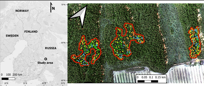
Fig. 1. The location of the study area (Jyrinvaara) in Finland (left), and a zoomed in view (right) of this protected area. Within the protected area, there are three old-growth forest parts containing European aspen that are outlined in red. The various colored dots represent the various tree species (green for European aspen, yellow for birches [both silver and downy birch], blue for Norway spruce, and orange for Scots pine).
Based on data collected in 2019 from the Ilomantsi Pötsönvaara weather station (63°14´N, 31°04´E; downloaded from https://en.ilmatieteenlaitos.fi/download-observations) the average temperature of the coldest month was –12 °C in January and of the warmest month +15.1 °C in June. Furthermore, the annual rainfall was 793.5 mm of which 43% fell as snow and the thermal growing season (defined to begin when the daily mean temperature rises above 5 °C and snow has melted from open areas and to end when the daily mean temperature falls permanently below 5 °C) lasted from 27 April until 17 September with a total of 1068.6 degree days.
Based on an earlier inventory of these protected areas (Kouki et al. 2004; Hardenbol et al. 2020), we selected the Jyrinvaara area for this study. It had a typical density of aspen of various sizes in its old-growth forest parts (Fig. 1). In this protected area we inventoried all the old-growth forest parts (three parts in total). The dominant tree species in this reserve are Norway spruce and Scots pine. Silver birch (Betula pendula Roth) and downy birch (B. Pubescens Ehrh.) are rather common, while less common species include aspen, rowan (Sorbus aucuparia L.), and grey alder (Alnus incana [L.] Moench). This taxonomy is based on the database from the Missouri Botanical Garden (2021). The size of the three inventoried old-growth forest parts was ca. 9 ha in total.
Within the reserve, both diameter at breast height (dbh) and position were recorded for all living aspens (n = 106) and for a sample of birches (n = 160) located close to aspens with a dbh above 5 cm in 2019 (Table 1). Dbh was measured at 1.3 m height above ground. The positions were recorded with a Topcon HiPer V and a Trimble R10 Global Navigation Satellite Systems (GNSS) with an accuracy of <1 m for horizontal coordinates. In a comparison with aerial images, it was clear that some trees had >2 m positioning errors. The clearly erroneous tree locations were later manually corrected based on RGB drone image mosaics to ensure a better match with the remotely sensed data. In addition, based on the RGB aerial images (see section 2.2), we visually selected pines (n = 122) and spruces (n = 122) to be included in the species classification (Supplementary file S1; Table 1). For these trees dbh was not available. The visual interpretation of pines and spruces was verified by two operators.
| Table 1. The reference trees for the training and validation of the remotely sensed models for aspen detection. The total number of trees per tree species and various diameter at breast height (dbh) measures are only available for the field-inventoried tree species. Birches refers to silver and downy birch. | |||||
| Tree species | Number of trees | Mean dbh (cm) | Minimum dbh (cm) | Maximum dbh (cm) | Data source |
| European aspen | 106 | 41 | 25 | 65 | Field |
| Birches | 160 | 28 | 17 | 44 | Field |
| Norway spruce | 122 | - | - | - | Visual interpretation |
| Scots pine | 122 | - | - | - | Visual interpretation |
2.2 Drone image data
The multispectral drone image data were acquired from the study area on five dates throughout the thermal growing season in 2019 (Table 2, Fig. 2). Our study included three acquisition dates at the beginning of the thermal growing season in spring, one in summer, and one in autumn. This skewed data acquisition was based on our hypothesis that springtime classification could potentially only be optimal during a limited period and we wanted to capture this moment while summer would be largely homogenous, and autumn would have a longer optimal timeframe. The images were acquired using a multi-rotor platform DJI Matrice 210 equipped with MicaSense RedEdge-M camera. The MicaSense sensor produces 1.2-megapixel images in the blue (B, 475 nm, full width at half maximum [FWHM] of 20 nm), green (G, 560 nm, FWHM of 20 nm), red (R, 668 nm, FWHM of 10 nm), red edge (RE, 717 nm, FWHM of 10 nm), and near infrared (NIR, 840 nm, FWHM of 40 nm) bands. The altitude of 135 m aboveground resulted in a ground sampling distance of around 9 cm. To avoid erroneous data due to changing illumination conditions during flight and to keep our data comparable between dates regardless of weather conditions (Table 2) we also collected data for later radiometric correction of the multispectral images. This data collection followed best practices as also outlined by MicaSense (2020). Immediately before and after each flight, we captured calibration images from a MicaSense Calibrated Reflectance Panel (CRP). The reflectance values of the CRP were: B = 0.528, G = 0.53, R = 0.53, RE = 0.53, and NIR = 0.528. Additionally, we equipped the drone with a RedEdge Downwelling Light Sensor (DLS) which attaches information about the illumination conditions to the metadata of every captured image during the flight.
| Table 2. Characteristics of the multispectral and RGB drone image data sets collected from our study area for aspen detection. | ||||||
| Date | Type | No. of images | Image overlap | Aspen developmental stage | Birch developmental stage | Weather condition |
| 13 May 2019 | Multispectral | 1339 | 80/75 | Leaf off | Late leaf flush | Sunny |
| 22 May 2019 | Multispectral | 1485 | 85/85 | Early leaf flush | Mature leaves | Overcast |
| 30 May 2019 | Multispectral | 1685 | 85/85 | Late leaf flush | Mature leaves | Sunny |
| 13 June 2019 | Multispectral | 1772 | 85/85 | Mature leaves | Mature leaves | Overcast |
| 27 Sept. 2019 | Multispectral | 1232 | 85/75 | Senescence | Senescence | Overcast |
| 27 Sept. 2019 | RGB | 1497 | 85/85 | Senescence | Senescence | Overcast |
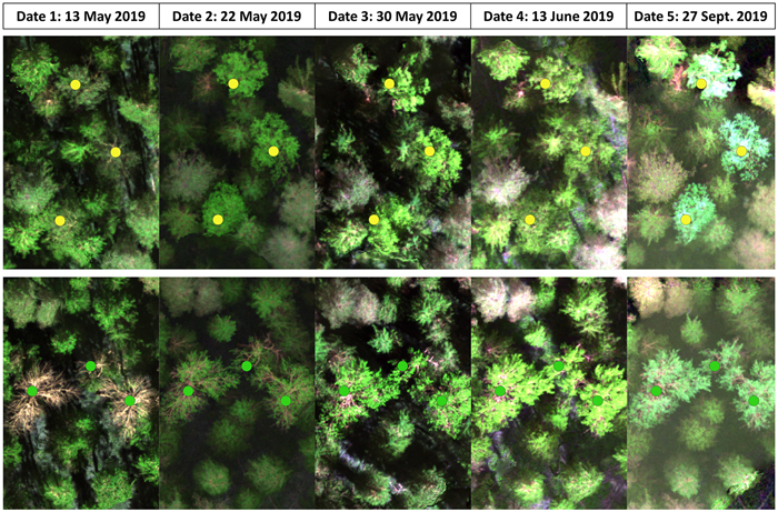
Fig. 2. False-color images from the five inventoried dates based on the collected multispectral data depicting the developmental stages of birches, both silver and downy birch (yellow dots) in the upper row and European aspen (green dots) in the bottom row.
We also collected RGB drone image data on date 5 (2019-09-27) for quality assurance, i.e. correction of wrongly positioned birches and aspens and segmentation accuracy assessment, and for adding the pines and spruces based on visual interpretation. These data were collected using a DJI Phantom 4 RTK multi-rotor platform with a real-time kinematic receiver and were processed into orthomosaics using the DJI software. The altitude of 140 m aboveground resulted in a ground sampling distance of 3.8 cm; compared with the 9 cm ground sampling distance of the multispectral data. Although multispectral data was tested for the purposes of quality assurance and for adding pines and spruces, the lower spatial resolution complicated these tasks.
We deployed four ground control points with white color cross targets of 50 by 50 cm to georeference the multispectral data. Their coordinates were measured using the virtual reference station real-time kinematic (VRS RTK) method with an accuracy of 1–2 cm for horizontal and vertical coordinates.
2.3 Image data processing
The drone data was processed to generate dense point clouds using the multispectral images. The processing was carried out using the Agisoft Metashape v. 1.6 software (Agisoft LLC, St. Petersburg, Russia) and followed the workflow outlined by Agisoft (2020). Agisoft Metashape is a commercial software that uses the Structure from Motion approach to generate a three-dimensional reconstruction from a collection of overlapping photographs, which can provide a dense and accurate three-dimensional point cloud (Iglhaut et al. 2019). The photogrammetric workflow consisted of three stages: radiometric correction, image alignment and point cloud densification. First, the calibration images taken from the CRP and the metadata info from the DLS were used for radiometric correction of the multispectral images by checking the Agisoft options “Use reflectance panels” and “Use sun sensor”. This resulted in calibrated reflectances that are less influenced by the weather conditions during data acquisition. In the second stage of processing, the quality was set to “high”, which means that full resolution images were used to orient the images. During this image alignment stage, camera calibration was also performed by Agisoft, based on Brown’s distortion model (Brown 1971). Finally, dense point clouds were calculated using the multispectral images to acquire the highest point density and resolution. During this stage, the software generates a photogrammetric point cloud based on the camera locations and orientations, and internal parameters determined by the “image alignment” stage. We selected “High quality” and “Moderate” as settings for “Quality” and “Depth filtering”, respectively, as these have been shown to be the most suitable settings for forest inventory (Puliti et al. 2015, 2017). The resultant point clouds included both xyz coordinates and spectral information for each point. The points were finally exported as text files for further processing.
2.4 Individual Tree Detection and computation of predictor variables
The multispectral photogrammetric point clouds from each date were processed separately. The points were first converted to the standard Finnish N2000 elevation system (Saaranen et al. 2021). The elevations were further normalized into above ground level with the publicly available ALS-based elevation model provided by the National Land Survey of Finland (2020). Subsequently, we outlined the inventoried old-growth forest parts (Fig. 1) and only used data that fell within these borders to reduce the computational cost. The points enveloped within the outlined area were tiled to further reduce computing demand. Each tile was 100 m, but a buffer of 10 m was added on each side to avoid splitting trees between tiles. Next, Canopy Height Models (CHMs) with a 50 cm resolution were constructed from the normalized point clouds using the LAStools software (Isenburg 2020) and the method presented by Isenburg (2014) and Khosravipour et al. (2014). This method avoids the generation of no-data areas inside the CHMs by stacking a set of temporary CHMs constructed with different height thresholds.
The ITD was performed with the R software version 3.5.3 (R Core Team 2019) and its libraries LidR (Roussel et al. 2020), rLiDAR (Silva et al. 2017), and ForestTools (Plowright and Roussel 2018). The CHMs were first smoothed with a Gaussian filter where the window size was five pixels. The smoothing intensity σ was set at 0.6 for pixels with height < 20 m and at 1.0 for pixels with height ≥ 20 m (Pitkänen et al. 2004). The locations and heights of the individual trees were first detected as local maxima in the CHMs based on a moving window with a size of 5 × 5 pixels. Local maxima with maximum height < 2 m were considered low vegetation and omitted.
Marker-controlled watershed segmentation was applied to the smoothed CHMs to obtain crown boundaries for each detected tree. Each boundary was linked with the largest field-measured tree within it. We did not measure all trees inside the study area, so a tree detection rate could not be assessed, but the accuracy of segmentation was evaluated visually against an orthomosaic produced from the RGB images. We examined how accurate the segments involving field-measured trees (only aspen and birch) were on date 5 (2019-09-27, Fig. 3). Highly accurate segments contained only one tree with only some branches from neighboring trees included. Moderately accurate segments contained a dominant tree that was properly linked to a field-measured tree but also contained some smaller distorting trees. Poorly accurate segments included multiple dominant trees and in many cases the field-measured tree was linked to a wrong dominant tree.
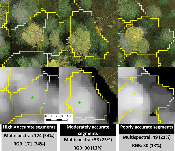
Fig. 3. Examples of highly, moderately, and poorly accurate automatic multispectral- and RGB-based segmentations and the number and percentage of segments in each accuracy category. The green dots represent European aspen, the yellow dot a silver birch, and the segments are outlined in yellow. The segmentation accuracies in this figure are from date 5 (2019-09-27). The pixel size is 3.3 cm.
Because the multispectral segmentation resulted in multiple poorly accurate segments that would have an effect on the interpretation of multi-seasonal data, we also executed the segmentation process in two alternate ways. First, we employed the processing chain described above for the RGB imagery available from 2019-09-27. These data provided a considerably higher point density, and fewer segments with moderate or poor accuracy. Second, we performed a manual segmentation based on an orthomosaic derived from the same RGB images. The segments were drawn in QGIS 3.16.5 (QGIS Development Team 2021) and verified by two operators. The manual segmentation was included as a best-case scenario that might be less useful in practice but would show the seasonal effects on classification without additional errors from segmentation.
Multispectral points with height ≥ 2 m above ground level were used to extract a set of spectral (n = 44) and height (n = 27) distribution variables for each tree segment (Table 3). The spectral values of each point were normalized by dividing the brightness at each band by the sum of all brightness values observed for the same point (Yu et al. 1999). All height percentiles as well as mean and median heights were normalized into relative values by dividing their values by the maximum height of the individual segments. Maximum height itself was not included as a predictor since it could not be normalized. This way the height distribution variables retained the information related to crown shape, but tree height did not have an effect in classification, which made the classification models more general. Finally, each predictor was normalized to the standard unit interval which made the model interpretation easier.
| Table 3. A list of all predictor variables for aspen detection that were extracted from the multispectral image point cloud data based on the individual tree segments. Abbreviations: H = height; R = red; G = green; B = blue; RE = red edge; NIR = near infrared; NDVI = normalized difference vegetation index; GNDVI = green normalized difference vegetation index. | |
| Predictors | Description |
| Height | |
| Relative H P5, H P10, …, H P95, H P99 | Height percentiles |
| Relative H Mean | Mean |
| Relative H Median | Median |
| H SD | Standard deviation |
| H Skew | Skewness |
| H Kurt | Kurtosis |
| H CV | Coefficient of variation |
| H VAR | Variance |
| Normalized spectral | |
| R;G;B;RE;NIR P5, R;G;B;RE;NIR P25, R;G;B;RE;NIR P75, R;G;B;RE;NIR P95 | Band percentiles |
| R;G;B;RE;NIR Mean | Mean |
| R;G;B;RE;NIR SD | Standard deviation |
| R;G;B;RE;NIR Skew | Skewness |
| R;G;B;RE;NIR Kurt | Kurtosis |
| NDVI;GNDVI P95* | NDVI and GNDVI 95% percentiles |
| NDVI;GNDVI Mean* | NDVI and GNDVI mean |
| * Equations: NDVI = (NIR – R)/(NIR + R) and GNDVI = (NIR – G)/(NIR + G) | |
2.5 Statistical analysis
The variables extracted for the segments that were linked with the field-measured trees were imported into R for species classification with linear discriminant analysis (LDA). We performed the LDA for two main classifications: (1) for separating all four tree species (four-class classification), and (2) for separating aspen against a combined class of birches, spruces, and pines (two-class classification). However, the results showed that the two-class case did not improve the accuracy of aspen inventory compared with the four-class case, so all results are reported for all species.
The LDA models were trained using the R-package MASS (Ripley et al. 2020). The number of predictor variables in the LDA was set at five, which is a compromise between the accuracy of predictions and avoidance of overfitting. We implemented the variable selection based on a heuristic optimization algorithm (Packalén et al. 2012) that is a modification of the original Simulated Annealing method (Kirkpatrick et al. 1983). This algorithm tested a large number of different predictor combinations attempting to improve from the best currently found predictor set. To avoid convergence on local optima in the variable space, worse solutions also had a probability to be accepted as the basis of further iterations. The probability of accepting worse solutions decreased linearly as the number of iterations increased and was controlled by a parameter called temperature. We iterated the algorithm ten thousand times with the temperature set as 0.2. The variable combination that provided the highest classification accuracy was selected for reporting. The accuracy was assessed based on two different criteria: (1) the greatest value of the summed user’s and producer’s accuracies of aspen, and (2) the greatest value of Cohen’s kappa coefficient. The first case provided the optimal variables for classifying aspen, and the second case for classification of all four tree species. For clarification, user’s accuracy is the accuracy from the user’s perspective and refers to how many of the trees predicted to belong to a certain species actually belong to that species. Conversely, producer’s accuracy is the accuracy from the producer’s perspective and refers to how many of the field-measured trees belonging to a certain species are correctly classified as that species (Congalton and Green 2019).
The reported accuracy values were obtained via leave-one-out cross-validation (LOOCV). The accuracy assessment was performed based on confusion matrices, overall/user’s/producer’s accuracies, and Cohen’s kappa coefficients. In addition, the discriminant functions and plots were interpreted to uncover the relative importance of different predictors. Discriminant functions are linear combinations that indicate how the various predictors determine the discriminant space where each observation is mapped to the nearest group center. Discriminant plots show how the various observations are scattered within this space. Our analysis mainly focused on the first two discriminants.
3 Results
3.1 Manual segmentation
3.1.1 Variable selection optimized for aspen
Manual segmentation yielded clearly higher classification accuracies than automatic segmentations in all cases, so we report its results first. When the variable selection was optimized for aspen separability, the user’s and producer’s accuracies for aspen ranged from 84% to 97% (Table 4). The accuracy of aspen classification was the greatest for date 1 (2019-05-13): user’s accuracy 97%, producer’s accuracy 96% (Table 4). At this time, the aspens were without leaves and the birches had partially flushed leaves. On date 1, aspen was separated by the first discriminant and the other species by the second discriminant (Fig. 4). The first discriminant separated aspen exceptionally well, but the other species showed clear overlap on the first discriminant. Both discriminants were dominated by spectral predictors (G P95, RE P95, RE P75, NDVI Mean) and the only relative height predictor (H P45) had a comparatively small effect on the classification (Table 5). Overall, the spectral predictors reflected the differences between aspens’ bare branches and the other species’ green leaves. The aspen group had the smallest group means for RE P95, RE P75, and NDVI Mean, as these predictors describe the amount of green vegetation. Aspen also had the largest group mean for G P95, because bare branches have larger reflectance at visible wavelengths than green vegetation. Interestingly, the RE P95 and RE P75 had different signs in the first discriminant (Table 5). We investigated the distributions of RE brightness values for crowns of different species, and for aspen the distribution was normal, while the other species’ distributions were left-skewed. This meant that aspen had a larger increase in brightness from RE P75 to RE P95 than other species, which could explain the differences in signs of these variables in the first discriminant function.
| Table 4. Accuracy values obtained from tree species classification by linear discriminant analysis and manual segmentation for the five inventoried dates. The best results obtained in the aspen- and kappa-optimized classifications are bolded. | ||||||
| Optimization criterion | Accuracy values | Date 1: 13 May 2019 | Date 2: 22 May 2019 | Date 3: 30 May 2019 | Date 4: 13 June 2019 | Date 5: 27 Sept. 2019 |
| Aspen-optimized | Kappa coefficient | 0.80 | 0.79 | 0.90 | 0.71 | 0.83 |
| Overall accuracy, % | 85 | 84 | 92 | 78 | 88 | |
| Aspen user’s accuracy, % | 97 | 85 | 96 | 84 | 87 | |
| Aspen producer’s accuracy, % | 96 | 95 | 93 | 91 | 84 | |
| Kappa-optimized | Kappa coefficient | 0.93 | 0.91 | 0.93 | 0.88 | 0.86 |
| Overall accuracy, % | 95 | 93 | 94 | 91 | 90 | |
| Aspen user’s accuracy, % | 96 | 90 | 92 | 85 | 86 | |
| Aspen producer’s accuracy, % | 96 | 83 | 94 | 84 | 83 | |
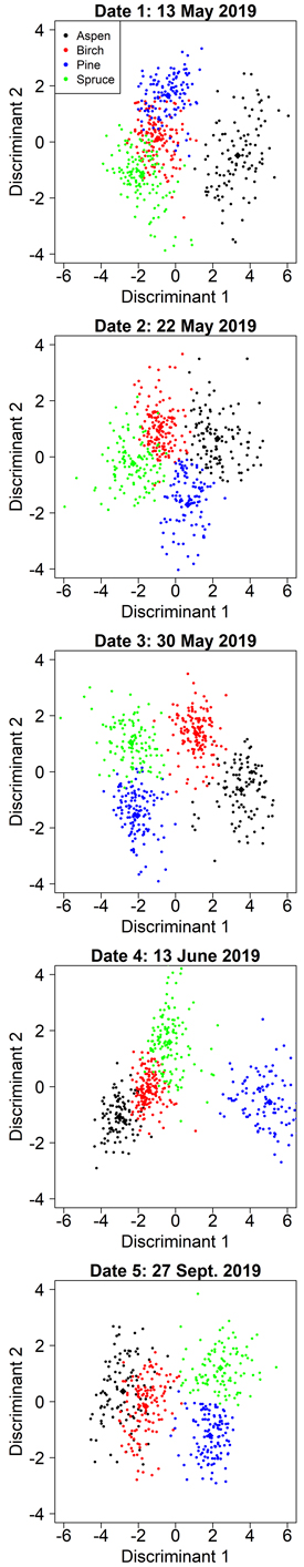
Fig. 4. Class separation by two discriminant axes in the aspen-optimized tree species classification by manual segmentation on the five inventoried dates.
| Table 5. The selected predictors, their normalized and non-normalized (in parentheses) means for all four tree species, and the discriminant function coefficients obtained from the aspen-optimized tree species classification by linear discriminant analysis and manual segmentation. The most important predictors for each discriminant and date are bolded. Abbreviations: P = Percentile; H = height; R = red; G = green; B = blue; RE = red edge; NIR = near infrared; NDVI = normalized difference vegetation index; GNDVI = green normalized difference vegetation index. Birches refers to silver and downy birch. | |||||||
| Dates | Predictors | Predictor means for European aspen | Predictor means for birches | Predictor means for Scots pine | Predictor means for Norway spruce | LD1 | LD2 |
| Date 1: 13 May 2019 | H P45 | 0.48 (0.85) | –0.06 (0.79) | 0.04 (0.80) | –0.37 (0.76) | 0.22 | –0.24 |
| G P95 | 1.34 (0.14) | –0.18 (0.12) | –0.19 (0.12) | –0.75 (0.12) | 0.61 | –1.34 | |
| RE P95 | –0.89 (0.27) | 0.79 (0.29) | –0.04 (0.28) | –0.13 (0.28) | 1.47 | –1.36 | |
| RE P75 | –1.12 (0.25) | 0.70 (0.28) | 0.23 (0.27) | –0.09 (0.26) | –2.28 | 1.86 | |
| NDVI Mean | –1.16 (0.64) | 0.16 (0.73) | –0.37 (0.69) | 1.17 (0.80) | –1.00 | –2.00 | |
| Date 2: 22 May 2019 | H P70 | 0.57 (0.91) | 0.23 (0.89) | 0.01 (0.88) | –0.76 (0.83) | 0.64 | 0.47 |
| NIR SD | 1.03 (0.05) | –0.42 (0.03) | 0.05 (0.04) | –0.43 (0.03) | 0.48 | 0.45 | |
| R Skew | –0.62 (0.19) | 0.84 (1.21) | –0.91 (–0.01) | 0.43 (0.92) | –0.14 | 1.59 | |
| RE Skew | 0.65 (–0.27) | –0.13 (–0.61) | –0.55 (–0.79) | 0.15 (–0.49) | –0.04 | 0.72 | |
| NIR P25 | –1.13 (0.41) | 0.41 (0.46) | –0.51 (0.43) | 0.98 (0.48) | –1.24 | –0.42 | |
| Date 3: 30 May 2019 | H P55 | 0.46 (0.85) | 0.11 (0.82) | 0.02 (0.81) | –0.54 (0.76) | 0.45 | –0.36 |
| B Kurt | –0.22 (2.14) | 0.81 (5.47) | –0.72 (0.50) | –0.07 (2.61) | 0.07 | 0.28 | |
| RE P95 | 1.16 (0.32) | 0.64 (0.31) | –0.91 (0.27) | –0.87 (0.27) | 4.45 | –0.25 | |
| B P75 | 0.35 (0.06) | –0.77 (0.05) | 1.08 (0.07) | –0.44 (0.05) | 0.25 | –1.33 | |
| RE P75 | 0.94 (0.30) | 0.73 (0.29) | –0.78 (0.26) | –0.91 (0.26) | –2.21 | 0.16 | |
| Date 4: 13 June 2019 | H P65 | –0.23 (0.01) | –0.01 (0.01) | –0.35 (0.01) | 0.56 (0.01) | –0.04 | –0.53 |
| R SD | 0.16 (0.02) | –0.34 (0.01) | 0.77 (0.02) | –0.50 (0.01) | –0.50 | 0.26 | |
| B P25 | –0.56 (0.04) | –0.56 (0.04) | 1.50 (0.06) | –0.33 (0.04) | 2.02 | 0.56 | |
| R P25 | –0.66 (0.04) | –0.53 (0.04) | 1.59 (0.08) | –0.37 (0.04) | –9.09 | –4.21 | |
| NDVI Mean | 0.52 (0.84) | 0.55 (0.84) | –1.53 (0.71) | 0.43 (0.83) | –4.49 | –3.70 | |
| Date 5: 27 Sept. 2019 | H P95 | 0.32 (0.97) | 0.33 (0.97) | –0.04 (0.96) | –0.63 (0.95) | –0.40 | –0.17 |
| NIR Skew | 0.72 (1.03) | 0.48 (0.86) | –0.02 (0.51) | –1.17 (–0.30) | –0.30 | –1.26 | |
| G P95 | 0.78 (0.14) | 0.69 (0.14) | –0.46 (0.13) | –1.04 (0.12) | –0.44 | –0.79 | |
| RE P95 | 1.10 (0.32) | 0.66 (0.31) | –0.95 (0.27) | –0.81 (0.27) | –3.51 | 1.49 | |
| RE P75 | 1.03 (0.30) | 0.72 (0.30) | –0.89 (0.26) | –0.87 (0.26) | 1.86 | 0.12 | |
The accuracy of aspen classification decreased when leaves were present on both aspen and birch (Table 4). However, date 3 (2019-05-30) showed nearly as good accuracies for aspen as date 1 (user’s 96%, producer’s 93%). On date 3, the first discriminant separated the aspen and birch from the conifers, primarily based on two RE variables (Table 5). The second discriminant established another axis where aspen and pine had small values while birch and spruce had large values. The second discriminant was dominated by B P75, where pine and aspen had larger group means than birch and spruce. The blue wavelengths are strongly absorbed by chlorophylls, so this observation could mean that birch and spruce were experiencing different developmental stages or had different levels of chlorophyll content in late May compared with pine and aspen.
The other dates showed clearly worse accuracies for aspen (user’s 84–87%, producer’s 84–91%) but overall, these values were still rather good (Table 4). Based on the confusion matrices (Suppl. file S2), mixing between aspen and birch occurred primarily at dates 4 (2019-06-13) and 5 (2019-09-27). On date 2, slight mixing between aspen and pine could also be observed. During the autumn season (date 5, 2019-09-27) when leaf coloration altered, there was a clear decline in aspen classification accuracy compared to spring and summer, and the greatest amount of mixing with birch. Spectral variables dominated the discriminant functions for each of these dates, and each model had only one relative height metric. Predictors derived from red edge or NIR bands were included in each model (Table 5), indicating that multispectral sensors provide considerably better accuracies in species classification than ordinary RGB cameras. Full confusion matrices for each date are shown in Suppl. file S2.
3.1.2 Variable selection optimized for kappa of all species
We also performed an alternative classification where the variable selection was optimized by the kappa coefficient obtained from LDA of all four species. The overall accuracy for all four species was relatively stable throughout the growing season and ranged from 90% to 95% (Table 4). The kappa coefficient on the other hand ranged from 0.86 to 0.93. The greatest accuracies were again obtained on dates 1 (2019-05-13, 95%) and 3 (2019-05-30, 94%).
On date 1, the classification model was comparable to the model with aspen-optimized predictors but relied solely on spectral data. The first discriminant was primarily influenced by red edge and near-infrared bands and contributed to the separation of pine and aspen (Table 6). The second discriminant focused primarily on separating birch (Fig. 5) and was dominated by the green band (G P75). Fig. 5 shows that the first two discriminants did not separate pine very well, but the third discriminant (not shown) contributed 13% to the total separation and primarily improved the classification of pine.
| Table 6. The selected predictors, their normalized and non-normalized (in parentheses) means for all four tree species, and the discriminant function coefficients obtained from the kappa-optimized tree species classification by linear discriminant analysis and manual segmentation. The most important predictors for each discriminant and date are bolded. Abbreviations: P = Percentile; H = height; R = red; G = green; B = blue; RE = red edge; NIR = near infrared; NDVI = normalized difference vegetation index; GNDVI = green normalized difference vegetation index. Birches refers to silver and downy birch. | |||||||
| Dates | Predictors | Predictor means for European aspen | Predictor means for birches | Predictor means for Scots pine | Predictor means for Norway spruce | LD1 | LD2 |
| Date 1: 13 May 2019 | G P95 | 1.34 (0.14) | –0.18 (0.12) | –0.19 (0.12) | –0.75 (0.12) | 0.91 | 1.43 |
| RE P95 | –0.89 (0.27) | 0.79 (0.29) | –0.04 (0.28) | –0.13 (0.28) | 1.44 | 0.10 | |
| G P75 | 1.21 (0.13) | –0.37 (0.11) | 0.15 (0.11) | –0.74 (0.11) | –1.81 | –4.20 | |
| RE P75 | –1.12 (0.25) | 0.70 (0.28) | 0.23 (0.27) | –0.09 (0.26) | –2.40 | 0.74 | |
| NIR P25 | –1.03 (0.43) | 0.04 (0.48) | –0.36 (0.46) | 1.19 (0.53) | –2.68 | –2.91 | |
| Date 2: 22 May 2019 | H P70 | 0.57 (0.91) | 0.23 (0.89) | 0.01 (0.88) | –0.76 (0.83) | –0.75 | –0.29 |
| NIR SD | 1.03 (0.05) | –0.42 (0.03) | 0.05 (0.04) | –0.43 (0.03) | –0.64 | –0.53 | |
| G P95 | 1.17 (0.14) | –0.07 (0.13) | –0.28 (0.13) | –0.64 (0.13) | –0.33 | 0.72 | |
| RE P95 | 0.18 (0.31) | 1.17 (0.33) | –0.80 (0.29) | –0.76 (0.29) | –1.71 | –0.18 | |
| R P25 | 0.76 (0.09) | –0.94 (0.06) | 1.00 (0.09) | –0.51 (0.06) | –0.19 | –2.07 | |
| Date 3: 30 May 2019 | H P55 | 0.46 (0.85) | 0.11 (0.82) | 0.02 (0.81) | –0.54 (0.76) | 0.34 | 0.47 |
| R Mean | 0.01 (0.06) | –0.80 (0.05) | 1.36 (0.08) | –0.40 (0.06) | –0.54 | 2.48 | |
| RE P95 | 1.16 (0.32) | 0.64 (0.31) | –0.91 (0.27) | –0.87 (0.27) | 4.29 | 1.24 | |
| NIR P75 | –0.32 (0.57) | 0.07 (0.58) | –0.48 (0.56) | 0.67 (0.61) | –0.22 | 0.97 | |
| RE P75 | 0.94 (0.30) | 0.73 (0.29) | –0.78 (0.26) | –0.91 (0.26) | –2.30 | –0.07 | |
| Date 4: 13 June 2019 | B Mean | –0.45 (0.04) | –0.58 (0.04) | 1.44 (0.06) | –0.35 (0.04) | –1.58 | –2.96 |
| G Mean | 0.22 (0.11) | –0.65 (0.10) | 0.74 (0.11) | –0.15 (0.10) | 0.30 | 3.26 | |
| RE P75 | 1.02 (0.27) | 0.38 (0.27) | –0.70 (0.26) | –0.63 (0.26) | –0.49 | –2.76 | |
| R P25 | –0.66 (0.04) | –0.53 (0.04) | 1.59 (0.08) | –0.37 (0.04) | 4.29 | –0.18 | |
| GNDVI P95 | –0.24 (0.66) | 0.42 (0.68) | –0.58 (0.65) | 0.28 (0.67) | 0.52 | 0.42 | |
| Date 5: 27 Sept. 2019 | H P70 | 0.45 (0.92) | 0.36 (0.91) | –0.04 (0.89) | –0.78 (0.85) | –0.60 | –0.07 |
| NIR SD | 0.64 (0.05) | 0.42 (0.05) | –0.30 (0.04) | –0.76 (0.03) | –0.52 | –0.12 | |
| RE P95 | 1.10 (0.32) | 0.66 (0.31) | –0.96 (0.27) | –0.81 (0.27) | –2.42 | 2.08 | |
| RE P75 | 1.03 (0.30) | 0.72 (0.30) | –0.89 (0.26) | –0.87 (0.26) | 0.33 | –2.92 | |
| B P25 | –0.39 (0.04) | –0.54 (0.03) | 1.49 (0.05) | –0.46 (0.03) | –0.21 | –2.10 | |
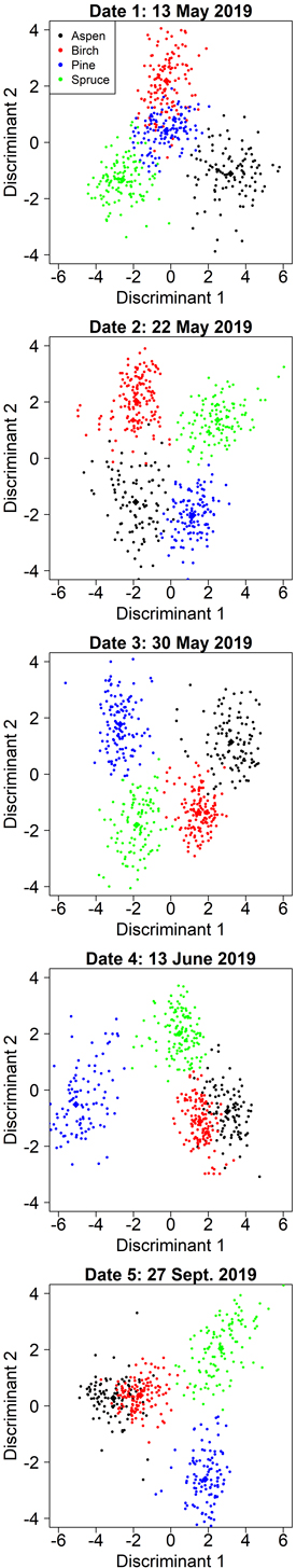
Fig. 5. Class separation by two discriminant axes in the kappa-optimized tree species classification by manual segmentation on the five inventoried dates.
On date 3, the selected model resembled the corresponding aspen-optimized model, but the separation of pine and spruce was improved by employing the red (R Mean) and near-infrared (NIR P75) bands instead of the previous predictors derived from the blue band. The lowest overall accuracy was obtained in the autumn (date 5, 2019-09-27), but was still very good at 90%. Pine, spruce, and the deciduous species were well separated both in summer (date 4, 2019-06-13) and autumn, but the mixing between aspen and birch at these dates decreased the overall accuracy (Fig. 5). Full confusion matrices for each date are shown in Suppl. file S3.
3.2 Comparison of manual and automatic segmentations
In contrast to the manual segmentation, the automatic multispectral-based and RGB-based segmentations resulted in lower classification accuracies for all dates and optimizations because of poorer segmentation (Table 7). The multispectral-based segmentation in the aspen-optimized classification had user’s accuracies for aspen ranging from 77% to 89% and producer’s accuracies ranging from 78% to 91%. Conversely, based on the RGB segmentation, the user’s accuracies for aspen ranged from 85% to 97% and producer’s accuracies ranged from 79% to 93%. Similarly, in the kappa-optimized classification, the classification based on the multispectral segmentation resulted in a kappa coefficient ranging from 0.75 to 0.81 while classification based on the RGB segmentation had a kappa coefficient ranging from 0.84 to 0.90. In agreement with the classification based on the manual segmentation, date 1 had the best results for aspen-optimized classifications based on automatic segmentation. In contrast, date 3 for multispectral-based segmentation and date 2 for RGB-based segmentation proved more accurate than date 1 in the kappa-optimized classification. It is important to note that the predictor selection differed considerably in the classifications based on automatic segmentation compared with the classifications based on the manual segmentation. As such, the classifications based on the automatic segmentations did not just add more random error with the same selected predictors, which can clearly be seen when comparing discriminant plots (Fig. 4 with Suppl. file S6 and Fig. 5 with Suppl. file S7). The selected predictors for each date with multispectral-based and RGB-based segmentation are shown in Suppl. files S4 and S5.
| Table 7. Tree species classification accuracy values obtained from both the aspen-optimized and the kappa-optimized variable selections based on multispectral-based and RGB-based segmentations. The best results in the aspen- and kappa-optimized classifications are bolded. | ||||||
| Optimization criterion | Accuracy values | Date 1: 13 May 2019 | Date 2: 22 May 2019 | Date 3: 30 May 2019 | Date 4: 13 June 2019 | Date 5: 27 Sept. 2019 |
| Multispectral-based segmentation | ||||||
| Aspen-optimized | Kappa coefficient | 0.55 | 0.52 | 0.80 | 0.65 | 0.72 |
| Overall accuracy, % | 66 | 64 | 85 | 74 | 79 | |
| Aspen user’s accuracy, % | 89 | 85 | 86 | 87 | 77 | |
| Aspen producer’s accuracy, % | 91 | 78 | 84 | 83 | 81 | |
| Kappa-optimized | Kappa coefficient | 0.77 | 0.78 | 0.81 | 0.79 | 0.75 |
| Overall accuracy, % | 83 | 84 | 86 | 84 | 81 | |
| Aspen user’s accuracy, % | 88 | 79 | 84 | 78 | 75 | |
| Aspen producer’s accuracy, % | 84 | 71 | 76 | 83 | 79 | |
| RGB-based segmentation | ||||||
| Aspen-optimized | Kappa coefficient | 0.70 | 0.80 | 0.89 | 0.71 | 0.83 |
| Overall accuracy, % | 78 | 85 | 91 | 79 | 87 | |
| Aspen user’s accuracy, % | 97 | 89 | 91 | 85 | 85 | |
| Aspen producer’s accuracy, % | 93 | 87 | 88 | 81 | 79 | |
| Kappa-optimized | Kappa coefficient | 0.84 | 0.90 | 0.88 | 0.84 | 0.85 |
| Overall accuracy, % | 88 | 92 | 91 | 88 | 89 | |
| Aspen user’s accuracy, % | 90 | 90 | 88 | 80 | 82 | |
| Aspen producer’s accuracy, % | 92 | 79 | 83 | 82 | 80 | |
As indicated above, the RGB-based segmentation resulted in better classification results than the multispectral-based segmentation and this is clearly a result of segmentation accuracy. In all cases, the RGB-based segmentation proved more accurate than the multispectral-based segmentation (Fig. 3). For example, on date 5 the RGB-based segmentation had 30 moderately and 30 poorly accurate segments while the multispectral-based segmentation had 58 moderately and 49 poorly accurate segments.
4 Discussion
4.1 Seasonal variations in aspen classification accuracy
Compared with previous efforts to separate aspen from other tree species, on the most optimal date with manual segmentation, we obtained excellent classification accuracies with a user’s accuracy of 97% and a producer’s accuracy of 96% for aspen. This result is comparable to the F1-scores of 92% for aspen reported by Viinikka et al. (2020) and the 86% reported by Kuzmin et al. (2021). Previously, however, the review by Kivinen et al. (2020) reported much lower accuracies for aspens classification with user’s accuracies between 56% and 86% and producer’s accuracies between 24% and 71%.
We find that spring, when aspen has no leaves yet, but birch already has leaves, is the optimal time to separate aspen from other tree species. This is likely a result of the differences in spectral values between bark or branches and leaves and indicates that there is little intraspecific variation in aspen and birch ecophysiology but there is large interspecific variation. Previous studies have also found or suggested that temporal differences in leaf flush can be used to separate tree species (Key et al. 2001; Persson et al. 2018). However, in other cases, large intraspecific variation can be a detriment despite obvious temporal differences in leaf flush (Lisein et al. 2015). The period during which aspen has no leaves but birch does is short and is probably under the influence of annual and geographic variation. Consequently, phenological monitoring via, for example, cameras mounted in place (Zeng et al. 2020) or drones (Fawcett et al. 2020) is required to not miss the optimal time for inventories.
During the late spring and summer season when both aspen and birches have leaves, there is little interspecific variation and strong spectral similarity between these tree species, and in addition intraspecific variation is small (Viinikka et al. 2020). Since this period lasts long, it is often selected for single date species classification studies. However, in accordance with other studies (Persson et al. 2018), we find that the lack of obvious phenological differences results in poorer classification accuracy of images acquired during summer. Like the study by Viinikka et al. (2020) we find that the red edge and near infrared bands are important to discriminate aspen during this time.
Despite expectations that the autumn senescence period would be a good time to separate aspen from the other tree species based on phenological differences (Hill et al. 2010; Persson et al. 2018), with our data this was the poorest performing time. Previous studies have shown both worse (Voss and Sugumaran 2008; Lisein et al. 2015) and better (Key et al. 2001; Hill et al. 2010) performance in species classification of deciduous trees in autumn compared with other periods. The poorer classification accuracy during the autumn senescence period in our case can potentially be attributed to the large degree of intraspecific variation in the onset of aspen senescence, even within local populations (Fracheboud et al. 2009). Leaf/canopy spectral values during the autumn senescence period are strongly connected to the onset timing (Lichtenthaler 1987) and since the onset displays large variation, canopy spectral values between aspen trees likely also portray large variation on a particular date throughout this period (Keskitalo et al. 2005). Furthermore, aside from senescence timing influencing spectral values there may also be inherent differences between aspen trees in their autumn coloration not influenced by the onset of senescence, especially between individuals from different clonal colonies. Intraspecific variation might be a bigger challenge in the autumn senescence period compared with other times of the year. Fracheboud et al. (2009) observed that in contrast to the onset of aspen autumn senescence, the onset of bud set in aspen exhibits much less variability within local populations. Our findings are, however, not conclusive on the value of images acquired in autumn, considering that we only had a single acquisition date in autumn and that the optimal autumn date may not have been covered by this acquisition. Moreover, leaf coloration during senescence can differ widely between years and thereby alter classification accuracy interannually (Hill et al. 2010).
4.2 Seasonal variations in overall classification accuracy
The accuracy values for all species are very promising, especially on the first and third date, with our findings presenting the best classification accuracy achieved thus far when considering aspen as a separate species (Viinikka et al. 2020). Our results suggest that the late spring/early summer season should be preferred in image acquisition for species-specific forest inventory scenarios. Focusing on the separability of pine and spruce, they were rather well separated on all dates but slightly worse in autumn. This is potentially related to annual ecophysiological patterns in pine whereby pine drops old needles in autumn and new shoots reach full size during summer (Hovi et al. 2016). Spruce, on the other hand, portrays less seasonal variation. Although we did not perform inventories in late summer (July and August), it is possible that pine and spruce separability performs worse with our method during that time, as observed by Hovi et al. (2016).
The separability of deciduous trees from conifers was most apparent on the third date. Seasonal variations in the separability of deciduous trees from conifers are likely related to combinations of the abovementioned seasonal ecophysiologies of the various tree species. Overall, we find that the red edge band is a reliable classifier for the separation of deciduous trees from conifers, in accordance with findings from hyperspectral datasets aimed at general tree species classification (reviewed by Fassnacht et al. 2016).
4.3 Implications for remote sensing
Our results showed that multispectral drone image point clouds have a great capability of detecting tree species, including non-dominant trees in mixed forests. Drones enable cost-effective data acquisitions for small-sized areas during the season that provides the best classification accuracy. The optimal time to acquire the images was late spring prior to aspen leaf flush for both aspen-optimized and general tree species classification. In Finland, springtime has already been shown to provide more accurate tree species estimates than other seasons, when airborne laser scanning data is used (Villikka et al. 2012; Hovi et al. 2016). Our results confirm that the same applies to drone image point clouds that also contain spectral information that is lacking from most laser scanning data sets. Predictors computed from the red edge and near infrared bands were repeatedly included into the various classification models. With advances in hyperspectral sensors, the accuracy of tree species classification could potentially be further improved (Sothe et al. 2019; Viinikka et al. 2020), but the higher spectral resolution comes at the cost of spatial resolution and geometric accuracy (Feng et al. 2020).
Using a multispectral sensor as a single-sensor solution to inventory aspens has proven relatively inaccurate in our case. The main problem was that the multispectral sensor had a larger ground sampling distance than the RGB sensor’s, which led to a less dense point cloud. As a result, also the accuracies of automatic segmentation and the resultant classification were poorer with multispectral data. The inaccuracy of the automatically produced segments meant that there were multiple cases in which several species were present within a single segment, and thus the spectral and height variables were skewed compared with more accurate manual or RGB-based segments. Thus, we recommend that additional RGB data from drone imagery acquired relatively close to the surface are also collected to obtain a more accurate segmentation. It is still beneficial to also process the multispectral images into point clouds because the introduction of height dimensions enables tree species classification using only points that are above a given height threshold. This way the confusing effect of ground pixels on the species classification can be avoided.
The classification accuracy of aspen was nevertheless still good with automatically produced segments for date 1 (multispectral-based segmentation: user’s 89%, producer’s 91%, RGB-based segmentation: user’s 97%, producer’s 93%). These are very promising results considering practical inventories in the future, especially if the accuracy of automatic segmentation can be improved further with higher resolution images and better segmentation algorithms. Manual segmentation is also a reasonable option in the model training stage, but applications to large-area mapping require automated segmentation approaches.
4.4 Implications for nature conservation
The importance of remote sensing applications for nature conservation (Kerr and Ostrovsky 2003; Nagendra et al. 2013) and especially the use of accurate tree species classification has been addressed multiple times (Shang and Chisholm 2014; Fassnacht et al. 2016). The importance of aspen classification is especially apparent for protected area designation (Lehtomäki et al. 2009) and the monitoring of aspen populations in established protected areas (Hardenbol et al. 2020). Our method resulted in a highly accurate and cost-effective way to provide general tree species classification as well as aspen-specific classification. However, since our study only included aspens that reach the canopy, complete demographic monitoring of aspen cohorts within a forest stand via remote sensing requires applications such as under-canopy drone laser scanning by which to classify below-canopy trees (Hyyppä et al. 2020). Despite this limitation in detecting individual below-canopy trees, we would recommend the use of our method for protected area designation and monitoring.
Declaration on the availability of research materials
Directly analyzable data, code, and digital research materials can be requested from the corresponding author. Other research materials are not available. No preregistration of either the study or the analysis plan took place.
Author contribution statement
Alwin A. Hardenbol*: Conceptualization, Methodology, Formal analysis, Investigation, Writing - Original Draft, Visualization, Project administration, Funding acquisition, Final approval.
Anton Kuzmin*: Conceptualization, Methodology, Investigation, Writing - Original Draft, Writing - Review & Editing, Final approval.
Lauri Korhonen: Conceptualization, Methodology, Formal analysis, Writing - Original Draft, Writing - Review & Editing, Supervision, Final approval.
Pasi Korpelainen: Conceptualization, Methodology, Writing - Original Draft, Investigation, Final approval.
Timo Kumpula: Conceptualization, Methodology, Investigation, Resources, Writing - Review & Editing, Supervision, Project administration, Funding acquisition, Final approval.
Matti Maltamo: Conceptualization, Methodology, Writing - Review & Editing, Final approval.
Jari Kouki: Conceptualization, Methodology, Writing - Review & Editing, Supervision, Funding acquisition, Project administration, Funding acquisition, Final approval.
* These authors contributed equally.
Acknowledgements
We would like to thank Aleksi Ritakallio and Max Stranden for their assistance with the field inventories. Adam Felton and Thibault Lachat are thanked for several comments that improved the manuscript.
Funding
This study was financially supported by the Maj and Tor Nessling foundation (AAH; grant number: 201700566), the Strategic Research Council at the Academy of Finland (TK; grant number 312559), and the Academy of Finland Flagship Programme (Forest-Human-Machine Interplay – Building Resilience, Redefining Value Networks and Enabling Meaningful Experiences (UNITE); grant number 337127), for which we kindly thank them. These funding sources had no further involvement besides funding our research.
References
Agisoft (2020) https://agisoft.freshdesk.com/support/solutions/articles/31000148780-micasense-rededge-mx-processing-workflow-including-reflectance-calibration-in-agisoft-metashape-pro. Accessed 20 January 2020.
Ahti T, Hämet-Ahti L, Jalas J (1968) Vegetation zones and their sections in northwestern Europe. Ann Bot Fenn 5: 169–211.
ArtDatabanken (2015) Rödlistade arter i Sverige 2015. [Red-listed species in Sweden 2015]. ArtDatabanken SLU, Uppsala, Sweden.
Berra EF, Gaulton R, Barr S (2019) Assessing spring phenology of a temperate woodland: a multiscale comparison of ground, unmanned aerial vehicle and Landsat satellite observations. Remote Sens Environ 223: 229–242. https://doi.org/10.1016/j.rse.2019.01.010.
Blackburn GA, Milton EJ (1995) Seasonal variations in the spectral reflectance of deciduous tree canopies. Int J Remote Sens 16: 709–720. https://doi.org/10.1080/01431169508954435.
Boyer M, Miller J, Belanger M, Hare E, Wu J (1988) Senescence and spectral reflectance in leaves of northern pin oak (Quercus palustris Muenchh.). Remote Sens Environ 25: 71–87. https://doi.org/10.1016/0034-4257(88)90042-9.
Brown DC (1971) Close-range camera calibration. Photogramm Eng 37: 855–866.
Chambers D, Périé C, Casajus N, de Blois S (2013) Challenges in modelling the abundance of 105 tree species in eastern North America using climate, edaphic, and topographic variables. Forest Ecol Manag 291: 20–29. https://doi.org/10.1016/j.foreco.2012.10.046.
Congalton RG, Green K (2019) Assessing the accuracy of remotely sensed data. Principles and practices 3rd edition. CRC Press, Florida, US. https://doi.org/10.1201/9780429052729.
Dalponte M, Ørka HO, Ene LT, Gobakken T, Næsset E (2014) Tree crown delineation and tree species classification in boreal forests using hyperspectral and ALS data. Remote Sens Environ 140: 306–317. https://doi.org/10.1016/j.rse.2013.09.006.
Dymond CC, Mladenoff DJ, Radeloff VC (2002) Phenological differences in Tasseled Cap indices improve deciduous forest classification. Remote Sens Environ 80: 460–472. https://doi.org/10.1016/S0034-4257(01)00324-8.
Erikson M (2004) Species classification of individually segmented tree crowns in high-resolution aerial images using radiometric and morphologic image measures. Remote Sens Environ 91: 469–477. https://doi.org/10.1016/j.rse.2004.04.006.
Esseen P-A, Ehnström B, Ericson L, Sjöberg K (1997) Boreal forests. Ecol Bull 46: 16–47.
Fassnacht FE, Latifi H, Stereńczak K, Modzelewska A, Lefsky M, Waser LT, Straub C, Ghosh A (2016) Review of studies on tree species classification from remotely sensed data. Remote Sens Environ 186: 64–87. https://doi.org/10.1016/j.rse.2016.08.013.
Fawcett D, Bennie J, Anderson K (2020) Monitoring spring phenology of individual tree crowns using drone-acquired NDVI data. Remote Sens Ecol Conserv 7: 227–244. https://doi.org/10.1002/rse2.184.
Feng X, He L, Cheng Q, Long X, Yuan Y (2020) Hyperspectral and multispectral remote sensing image fusion based on endmember spatial information. Remote Sens 12, article id 1009. https://doi.org/10.3390/rs12061009.
Fracheboud Y, Luquez V, Björkén L, Sjödin A, Tuominen H, Jansson S (2009) The control of autumn senescence in European aspen. Plant Physiol 149: 1982–1991. https://doi.org/10.1104/pp.108.133249.
Franklin SE, Ahmed OS (2018) Deciduous tree species classification using object-based analysis and machine learning with unmanned aerial vehicle multispectral data. Int J Remote Sens 39: 5236–5245. https://doi.org/10.1080/01431161.2017.1363442.
Hardenbol AA, Junninen K, Kouki J (2020) A key tree species for forest biodiversity, European aspen (Populus tremula), is rapidly declining in boreal old-growth forest reserves. Forest Ecol Manag 462, article id 118009. https://doi.org/10.1016/j.foreco.2020.118009.
Heide OM (1993) Daylength and thermal time responses of budburst during dormancy release in some northern deciduous trees. Physiol Plantarum 88: 531–540. https://doi.org/10.1111/j.1399-3054.1993.tb01368.x.
Henriksen S, Hilmo O (2015) Norsk rødliste for arter 2015. [Norwegian red list of species 2015]. Artsdatabanken, Norway.
Hill RA, Wilson AK, George M, Hinsley SA (2010) Mapping tree species in temperate deciduous woodland using time-series multi-spectral data. Appl Veg Sci 13: 86–99. https://doi.org/10.1111/j.1654-109X.2009.01053.x.
Holmgren J, Persson Å, Söderman U (2008) Species identification of individual trees by combining high resolution LiDAR data with multi‐spectral images. Int J Remote Sens 29: 1537–1552. https://doi.org/10.1080/01431160701736471.
Hovi A, Korhonen L, Vauhkonen J, Korpela I (2016) LiDAR waveform features for tree species classification and their sensitivity to tree- and acquisition related parameters. Remote Sens Environ 173: 224–237. https://doi.org/10.1016/j.rse.2015.08.019.
Hyvärinen E, Juslén A, Kemppainen E, Uddström A, Liukko U-M (2019) The 2019 red list of Finnish species. Ympäristöministeriö & Suomen ympäristökeskus, Helsinki, Finland. http://hdl.handle.net/10138/299501.
Hyyppä E, Hyyppä J, Hakala T, Kukko A, Wulder MA, White JC, Pyörälä J, Yu X, Wang Y, Virtanen J-P, Pohjavirta O, Liang X, Holopainen M, Kaartinen H (2020) Under-canopy UAV laser scanning for accurate forest field measurements. ISPRS J of Photogramm 164: 41–60. https://doi.org/10.1016/j.isprsjprs.2020.03.021.
Iglhaut J, Cabo C, Puliti S, Piermattei L, O’Connor J, Rosette J (2019) Structure from motion photogrammetry in forestry: a review. Curr For Rep 5: 155–168. https://doi.org/10.1007/s40725-019-00094-3.
Isenburg M (2014) Rasterizing perfect Canopy Height Models from LiDAR. https://rapidlasso.com/2014/11/04/rasterizing-perfect-canopy-height-models-from-lidar/. Accessed 12 August 2020.
Isenburg M (2020) LAStools – efficient LiDAR processing software, version 200509, academic license. https://rapidlasso.com/LAStools/.
Kerr JT, Ostrovsky M (2003) From space to species: ecological applications for remote sensing. Trends Ecol Evol 18: 299–305. https://doi.org/10.1016/S0169-5347(03)00071-5.
Keskitalo J, Bergquist G, Gardeström P, Jansson S (2005) A cellular timetable of autumn senescence. Plant Physiol 139: 1635–1648. https://doi.org/10.1104/pp.105.066845.
Key T, Warner TA, McGraw JB, Fajvan MA (2001) A comparison of multispectral and multitemporal information in high spatial resolution imagery for classification of individual tree species in a temperate hardwood forest. Remote Sens Environ 75: 100–112. https://doi.org/10.1016/S0034-4257(00)00159-0.
Khosravipour A, Skidmore AK, Isenburg M, Wang TJ, Hussin YA (2014) Generating pit-free Canopy Height Models from airborne LiDAR. Photogramm Eng and Rem S 80: 863–872. https://doi.org/10.14358/PERS.80.9.863.
Kirkpatrick S, Gelatt CD, Vecchi MP (1983) Optimization by simulated annealing. Science 220: 671–680. https://doi.org/10.1126/science.220.4598.671.
Kivinen S, Koivisto E, Keski-Saari S, Poikolainen L, Tanhuanpää T, Kuzmin A, Viinikka A, Heikkinen RK, Pykälä J, Virkkala R, Vihervaara P, Kumpula T (2020) A keystone species, European aspen (Populus tremula L.), in boreal forests: ecological role, knowledge needs and mapping using remote sensing. Forest Ecol Manag 462, article id 118008. https://doi.org/10.1016/j.foreco.2020.118008.
Korhonen KT, Tomppo E, Henttonen H, Ihalainen A, Tonteri T, Tuomainen T (2001) Pohjois-Karjalan metsäkeskuksen alueen metsävarat 1996–2000. [Forest resources in the North Karelia Forest Center area 1996–2000]. Metsätieteen Aikakauskirja 3B, article id 5861. https://doi.org/10.14214/ma.5861.
Korpela I, Ørka H, Maltamo M, Tokola T, Hyyppä J (2010) Tree species classification using airborne LiDAR – effects of stand and tree parameters, downsizing of training set, intensity normalization, and sensor type. Silva Fenn 44: 319–339. https://doi.org/10.14214/sf.156.
Kouki J, Arnold K, Martikainen P (2004) Long-term persistence of aspen – a key host for many threatened species – is endangered in old-growth conservation areas in Finland. J Nat Conserv 12: 41–52. https://doi.org/10.1016/j.jnc.2003.08.002.
Kuzmin A, Korhonen L, Kivinen S, Hurskainen P, Korpelainen P, Tanhuanpää T, Maltamo M, Vihervaara P, Kumpula T (2021) Detection of European aspen (Populus tremula L.) based on an unmanned aerial vehicle approach in boreal forests. Remote Sensing 13, article id 1723. https://doi.org/10.3390/rs13091723.
Lehtomäki J, Tomppo E, Kuokkanen P, Hanski I, Moilanen A (2009) Applying spatial conservation prioritization software and high-resolution GIS data to a national-scale study in forest conservation. Forest Ecol Manag 258: 2439–2449. https://doi.org/10.1016/j.foreco.2009.08.026.
Lehtonen H, Huttunen P (1997) History of forest fires in eastern Finland from the fifteenth century AD – the possible effects of slash-and-burn cultivation. The Holocene 7: 223–228. https://doi.org/10.1177/095968369700700210.
Lichtenthaler HK (1987) Chlorophyll fluorescence signatures of leaves during the autumnal chlorophyll breakdown. Journal of Plant Physiol 131: 101–110. https://doi.org/10.1016/S0176-1617(87)80271-7.
Lisein J, Michez A, Claessens H, Lejeune P (2015) Discrimination of deciduous tree species from time series of unmanned aerial system imagery. PLoS One 10, article id e0141006. https://doi.org/10.1371/journal.pone.0141006.
Mäyrä J, Keski-Saari S, Kivinen S, Tanhuanpää T, Hurskainen P, Kullberg P, Poikolainen L, Viinikka A, Tuominen S, Kumpula T, Vihervaara P (2021) Tree species classification from airborne hyperspectral and LiDAR data using 3D convolutional neural networks. Remote Sens Environ 256, article id 112322. https://doi.org/10.1016/j.rse.2021.112322.
MicaSense (2020) https://micasense.com/lets-talk-about-calibration/. Accessed 10 May 2021.
Michez A, Piégay H, Lisein J, Claessens H, Lejeune P (2016) Classification of riparian forest species and health condition using multi-temporal and hyperspatial imagery from unmanned aerial system. Environ Monit Assess 188, article id 146. https://doi.org/10.1007/s10661-015-4996-2.
Ministry of the Environment of Finland (1992) Vanhojen metsien suojelu valtion mailla etelä-Suomessa. [Protection programme for old-growth forests in southern Finland]. Report N-70. Ympäristöministeriö, Helsinki, Finland.
Ministry of the Environment of Finland (1994) Vanhojen metsien suojeluohjelman täydennys Etelä-Suomessa. [Protection programme for old-growth forests in southern Finland, additions]. Report N-2. Ympäristöministeriö, Helsinki, Finland.
Missouri Botanical Garden (2021) https://www.tropicos.org. Accessed 25 January 2021.
Nagendra H, Lucas R, Honrado JP, Jongman RHG, Tarantino C, Adamo M, Mairota P (2013) Remote sensing for conservation monitoring: assessing protected areas, habitat extent, habitat condition, species diversity, and threats. Ecol Indic 33: 45–59. https://doi.org/10.1016/j.ecolind.2012.09.014.
National Land Survey of Finland (2020) https://tiedostopalvelu.maanmittauslaitos.fi/tp/kartta?lang=en. Accessed 10 January 2020.
Nevalainen O, Honkavaara E, Tuominen S, Viljanen N, Hakala T, Yu X, Hyyppä J, Saari H, Pölönen I, Imai NN, Tommaselli AMG (2017) Individual tree detection and classification with UAV-based photogrammetric point clouds and hyperspectral imaging. Remote Sensing 9, article id 185. https://doi.org/10.3390/rs9030185.
Oldén A, Ovaskainen O, Kotiaho JS, Laaka-Lindberg S, Halme P (2014) Bryophyte species richness on retention aspens recovers in time but community structure does not. PLoS One 9, article id e93786. https://doi.org/10.1371/journal.pone.0093786.
Ørka HO, Næsset E, Bollandsås OM (2007) Utilizing airborne laser intensity for tree species classification. Int Arch Photogramm Remote Sens Spat Inf Sci 36, article id W52.
Ørka HO, Næsset E, Bollandsås OM (2009) Classifying species of individual trees by intensity and structure features derived from airborne laser scanner data. Remote Sens Environ 113: 1163–1174. https://doi.org/10.1016/j.rse.2009.02.002.
Packalén P, Temesgen H, Maltamo M (2012) Variable selection strategies for nearest neighbor imputation methods used in remote sensing based forest inventory. Can J Remote Sens 38: 557–569. https://doi.org/10.5589/m12-046.
Persson M, Lindberg E, Reese H (2018) Tree species classification with multi-temporal Sentinel-2 data. Remote Sens 10, article id 1794. https://doi.org/10.3390/rs10111794.
Pitkänen J, Maltamo M, Hyyppä J, Yu X (2004) Adaptive methods for individual tree detection on airborne laser based canopy height model. Int Arch Photogramm Remote Sens Spat Inf Sci 36: 187–191.
Plowright A, Roussel J-R (2018) ForestTools: analyzing remotely sensed forest data. https://CRAN.R-project.org/package=ForestTools.
Puliti S, Ørka HO, Gobakken T, Næsset E (2015) Inventory of small forest areas using an unmanned aerial system. Remote Sens 7: 9632–9654. https://doi.org/10.3390/rs70809632.
Puliti S, Gobakken T, Ørka HO, Næsset E (2017) Assessing 3D point clouds from aerial photographs for species-specific forest inventories. Scand J Forest Res 32: 68–79. https://doi.org/10.1080/02827581.2016.1186727.
QGIS Development Team (2021) QGIS Geographic Information System. Open Source Geospatial Foundation Project, Oregon, United States. https://www.qgis.org/.
R Core Team (2019) R: a language and environment for statistical computing. https://www.R-project.org/.
Ripley B, Venables B, Bates DM, Hornik K, Gebhardt A, Firth D (2020) MASS: support functions and datasets for venables and Ripley’s MASS. https://cran.r-project.org/package=MASS.
Roussel J-R, Auty D, de Boissieu F, Meador AS, Bourdon J-F, Gatziolis D (2020) lidR: airborne LiDAR data manipulation and visualization for forestry applications. https://cran.r-project.org/package=lidR.
Saaranen V, Lehmuskoski P, Takalo M, Rouhiainen P (2021) The third precise leveling of Finland. FGI publications 161. Finnish Geospatial Research Institute FGI, Kirkkonummi, Finland. http://hdl.handle.net/10138/326007.
Säynäjoki R, Packalén P, Maltamo M, Vehmas M, Eerikäinen K (2008) Detection of aspens using high resolution aerial laser scanning data and digital aerial images. Sensors 8: 5037–5054. https://doi.org/10.3390/s8085037.
Shang X, Chisholm LA (2014) Classification of Australian native forest species using hyperspectral remote sensing and machine-learning classification algorithms. IEEE J Sel Top Appl 7: 2481–2489. https://doi.org/10.1109/JSTARS.2013.2282166.
Sheeren D, Fauvel M, Josipović V, Lopes M, Planque C, Willm J, Dejoux J-F (2016) Tree species classification in temperate forests using Formosat-2 satellite image time series. Remote Sens 8, article id 734. https://doi.org/10.3390/rs8090734.
Silva CA, Crookston NL, Hudak AT, Vierling LA, Klauberg C, Cardil A (2017) rLiDAR: LiDAR data processing and visualization. https://cran.r-project.org/package=rLiDAR.
Sothe C, Dalponte M, de Almeida CM, Schimalski MB, Lima CL, Liesenberg V, Miyoshi GT, Tommaselli AMG (2019) Tree species classification in a highly diverse subtropical forest integrating UAV-based photogrammetric point cloud and hyperspectral data. Remote Sens 11, article id 1338. https://doi.org/10.3390/rs11111338.
Tikkanen O-P, Martikainen P, Hyvärinen E, Junninen K, Kouki J (2006) Red-listed boreal forest species of Finland: associations with forest structure, tree species, and decaying wood. Ann Zool Fenn 43: 373–383.
Tuominen S, Näsi R, Honkavaara E, Balazs A, Hakala T, Viljanen N, Pölönen I, Saari H, Ojanen H (2018) Assessment of classifiers and remote sensing features of hyperspectral imagery and stereo-photogrammetric point clouds for recognition of tree species in a forest area of high species diversity. Remote Sens 10, article id 714. https://doi.org/10.3390/rs10050714.
Uotila A, Kouki J, Kontkanen H, Pulkkinen P (2002) Assessing the naturalness of boreal forests in eastern Fennoscandia. Forest Ecol Manag 161: 257–277. https://doi.org/10.1016/S0378-1127(01)00496-0.
van Ewijk KY, Randin CF, Treitz PM, Scott NA (2014) Predicting fine-scale tree species abundance patterns using biotic variables derived from LiDAR and high spatial resolution imagery. Remote Sens Environ 150: 120–131. https://doi.org/10.1016/j.rse.2014.04.026.
Viinikka A, Hurskainen P, Keski-Saari S, Kivinen S, Tanhuanpää T, Mäyrä J, Poikolainen L, Vihervaara P, Kumpula T (2020) Detecting European aspen (Populus tremula L.) in boreal forests using airborne hyperspectral and airborne laser scanning data. Remote Sens 12, article id 2610. https://doi.org/10.3390/rs12162610.
Villikka M, Packalén P, Maltamo M (2012) The suitability of leaf-off airborne laser scanning data in an area-based forest inventory of coniferous and deciduous trees. Silva Fenn 46: 99–110. https://doi.org/10.14214/sf.68.
Voss M, Sugumaran R (2008) Seasonal effect on tree species classification in an urban environment using hyperspectral data, LiDAR, and an object-oriented approach. Sensors 8: 3020–3036. https://doi.org/10.3390/s8053020.
Weil G, Lensky IM, Resheff YS, Levin N (2017) Optimizing the timing of unmanned aerial vehicle image acquisition for applied mapping of woody vegetation species using feature selection. Remote Sens 9, article id 1130. https://doi.org/10.3390/rs9111130.
Xu Z, Shen X, Cao L, Coops NC, Goodbody TRH, Zhong T, Zhao W, Sun Q, Ba S, Zhang Z, Wu X (2020) Tree species classification using UAS-based digital aerial photogrammetry point clouds and multispectral imageries in subtropical natural forests. Int J Appl Earth Obs 92, article id 102173. https://doi.org/10.1016/j.jag.2020.102173.
Yu B, Ostland M, Gong P, Pu R (1999) Penalized discriminant analysis of in situ hyperspectral data for conifer species recognition. IEEE T Geosci Remote 37: 2569–2577. https://doi.org/10.1109/36.789651.
Zeng L, Wardlow BD, Xiang D, Hu S, Li D (2020) A review of vegetation phenological metrics extraction using time-series, multispectral satellite data. Remote Sens Environ 237, article id 111511. https://doi.org/10.1016/j.rse.2019.111511.
Total of 82 references.
