Mikko T. Niemi 
Improvements to stream extraction and soil wetness mapping within a forested catchment by increasing airborne LiDAR data density – a case study in Parkano, western Finland
Niemi M. T. (2021). Improvements to stream extraction and soil wetness mapping within a forested catchment by increasing airborne LiDAR data density – a case study in Parkano, western Finland. Silva Fennica vol. 55 no. 5 article id 10557. https://doi.org/10.14214/sf.10557
Highlights
- Overland flow routing can be improved with high-density airborne LiDAR data
- Kriging and inverse-distance weighting outperformed triangulated irregular networks in DEM interpolation
- A hybrid breaching-filling workflow performed well for DEM conditioning in the Finnish landscape
- Enhanced stream extraction and soil wetness mapping contribute to multi-purpose precision forestry.
Abstract
The pulse density of airborne Light Detection and Ranging (LiDAR) is increasing due to technical developments. The trade-offs between pulse density, inventory costs, and forest attribute measurement accuracy are extensively studied, but the possibilities of high-density airborne LiDAR in stream extraction and soil wetness mapping are unknown. This study aimed to refine the best practices for generating a hydrologically conditioned digital elevation model (DEM) from an airborne LiDAR -derived 3D point cloud. Depressionless DEMs were processed using a stepwise breaching-filling method, and the performance of overland flow routing was studied in relation to a pulse density, an interpolation method, and a raster cell size. The study area was situated on a densely ditched forestry site in Parkano municipality, for which LiDAR data with a pulse density of 5 m–2 were available. Stream networks and a topographic wetness index (TWI) were derived from altogether 12 DEM versions. The topological database of Finland was used as a ground reference in comparison, in addition to 40 selected main flow routes within the catchment. The results show improved performance of overland flow modeling due to increased data density. In addition, commonly used triangulated irregular networks were clearly outperformed by universal kriging and inverse-distance weighting in DEM interpolation. However, the TWI proved to be more sensitive to pulse density than an interpolation method. Improved overland flow routing contributes to enhanced forest resource planning at detailed spatial scales.
Keywords
remote sensing;
interpolation;
laser scanning;
digital elevation model conditioning;
overland flow routing;
soil drainage;
wetness index
-
Niemi,
Department of Forest Sciences, University of Helsinki, FI-00014 University of Helsinki, Finland
E-mail
mikko.t.niemi@helsinki.fi
Received 10 May 2021 Accepted 8 December 2021 Published 16 December 2021
Views 75287
Available at https://doi.org/10.14214/sf.10557 | Download PDF

Supplementary Files
1 Introduction
1.1 Motivation
Airborne Light Detection and Ranging (LiDAR) is an established data acquisition method for mapping soil and vegetation properties. LiDAR inventory generates a 3D point cloud of the environment, which may be used, for example, to interpolate a digital elevation model (DEM; Kraus and Pfeifer 1998; Sharma et al. 2020), to predict natural hazards (Jaboyedoff et al. 2012; Muhadi et al. 2020), and to estimate various forest attributes (Maltamo et al. 2014). Airborne LiDAR outperforms photogrammetry in elevation modeling thanks to the capacity of LiDAR beams to pass through forest canopy and reflect from ground level to a sensor (Kanostrevac et al. 2019).
The National Land Survey of Finland (NLS) has organized a nationwide acquisition of airborne LiDAR data for the purposes of land surveying and forest inventory using a pulse density of approximately 0.5 m–2. The pulse density was increased to 5 m–2 since summer 2020 (NLS 2021a), which enables increased accuracy in forest attribute estimates (Jakubowski et al. 2013). This provides a globally interesting setup for experiments due to a high initial point density and a wide dataset.
The links between LiDAR pulse density and measurement accuracy of terrain and forest properties have most often been assessed with respect to the success of deriving forest attributes, such as tree height (Maguya 2015). However, the advantage of increased pulse density should also be studied with respect to the performance of overland flow routing and wetness indices, which have major roles in hydrological processes and planning of peatland forestry (Launiainen et al. 2019). In addition, flow accumulation at catchment level can be utilized in different applications such as mapping wet soils (Lidberg et al. 2020), low terrain trafficability (Niemi et al. 2017; Salmivaara et al. 2020), erosion vulnerability (Frizzle et al. 2021), and augmenting forest growth models (Mohamedou et al. 2017).
1.2 Research needs, earlier knowledge, and objectives
GIS-based computation of continuous surface runoff and brook/ditch water flow demands a depressionless digital landscape. However, flow routing is particularly difficult close to anthropogenically modified terrain features such as roads and ditches because they manipulate natural flow paths and may create artificial sinks to DEM (Duke et al. 2006). Therefore, it is justified to test the success of DEM interpolation and subsequent computational flow accumulation in a relatively flat drained peatland area for discovering the entire potential of increasing airborne LiDAR data density.
An elevation model is the primary data source in flow routing algorithms (Wilson et al. 2008). The process of generating DEM from 3D point cloud requires two steps: firstly, ground points are classified from all LiDAR returns, and secondly, the DEM raster is interpolated from ground observations. The slope-based ground points filtering (Vosselman 2000) has been a main technique in point classification. Several interpolation methods, such as triangulated irregular network (TIN), inverse-distance weighting (IDW), natural neighbor, spline, minimum curvature, and universal kriging, have been applied and compared for generating elevation models. According to several earlier studies, kriging is the most accurate option for DEM interpolation (Heritage et al. 2009; Guo et al. 2010; Arun 2013).
Despite the filtering and interpolation choices, DEM rasters unavoidably contain local depressions without any downward direction (Jenson and Domingue 1988). Depressions are problematic in computational overland flow routing, as they affect discontinuity in flow network by accumulating water (Lindsay and Creed 2005). Depressionless DEM may be achieved either by filling depressions (O’Callaghan and Mark 1984; Wang and Liu 2006) or by breaching flow paths through barriers (Martz and Garbrecht 1998; Martz and Garbrecht 1999). The whole process of manipulating a depressionless elevation model is called DEM conditioning (Woodrow et al. 2016).
Previous studies of DEM conditioning have concluded that breaching should be the primary option, as it simulates culverts under bridges (Lindsay and Dhun 2015), and the real stream network was modelled significantly better in the Swedish landscape when using breaching instead of filling (Lidberg et al. 2017). If stream and ditch locations are known, the digitized stream network can be burned to the DEM raster before applying more robust filling or breaching algorithms (Lidberg et al. 2017). However, burning causes the risk of parallel stream segments if stream vector location differs from reality (Callow et al. 2007).
The development of overland flow routing methods has proceeded from a single-flow-direction algorithm (O’Callaghan and Mark 1984) towards a multiple-flow-direction (MFD) algorithm (Quinn et al. 1991; Holmgren 1994; Seibert and McGlynn 2007). The MFD method allows flow distribution to every possible downhill direction and gives more realistic information of soil wetness at landscape level (Pei et al. 2010). A flow accumulation grid can be utilized for various purposes, such as extracting a stream network (Murphy et al. 2008) or calculating wetness indices such as Topographic Wetness Index (TWI; Tarboton 1997) and Depth-to-water Index (DTW; Murphy et al. 2007). Both above-mentioned wetness estimates have provided promising results in boreal climate conditions (Murphy et al. 2009; Ågren et al. 2014).
This paper analyzes DEMs interpolated from high- and low-density airborne LiDAR data to refine best practices related to the acquisition and processing of 3D point data for overland flow routing within a forested catchment. The challenge and needs are global, but the Finnish landscape offers a fitting setting for implementing this study in a cost-efficient way, as fairly good information already exists on streams and man-made ditches, and detailed LiDAR point data are publicly available.
2 Materials and methods
2.1 Materials
The NLS Finland, responsible for organizing laser scanning campaigns, hosting data, maintaining, and developing a nationwide ground elevation model, and sharing all spatial data to further users with extensive usage permissions, implemented a high-density airborne LiDAR inventory for 20 production areas in summer 2020. The catchment of lake Kovesjärvi (62°04´N 22°50´E), covering approximately 20 km2 of land in one of the production areas (Fig. 1), was selected for further investigation because the surrounding forestland is densely ditched, and the topography is representative of the landscape in western Finland. In total, 220 km of streams and ditches within this catchment have been digitized to the topographical database of Finland by the NLS (2021b).
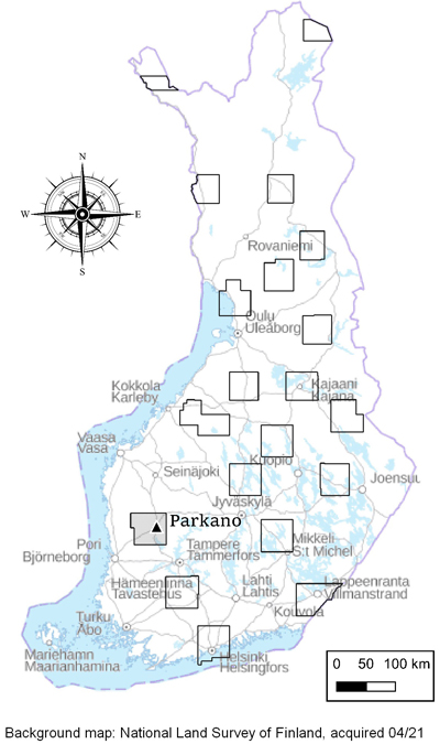
Fig. 1. The coverage of high-density airborne LiDAR data after inventories in 2020. The study of improving stream extraction and soil wetness mapping by increasing LiDAR data density was implemented in the catchment of lake Kovesjärvi (62°04´N, 22°50´E), which is located in Parkano municipality, roughly 240 km northwest of Helsinki, Finland.
The LiDAR inventory of Parkano production area was carried out in June 2020 by BSF Swissphoto AG, using a RIEGL VQ-1560i scanner. Flight altitude was 1525 meters and mean vertical error of observations should be less than 10 cm according to the data provider. The complete high-density (5 pulses m–2) LiDAR data are licensed and charged, but a thinned point data (0.5 pulses m–2), which is comparable to previous nationwide inventories, is shared freely for further users.
2.2 Methods
The LiDAR point data were classified by the data provider into several classes, such as ground, low vegetation, medium vegetation, and high vegetation points (NLS 2021a). A few classification parameters were tested using the LidarGroundPointFilter tool of WhiteboxTools (WBT) version 1.4.0 (Lindsay 2020) by varying the search radius and slope thresholds, and repeating the following workflow, but no improvement was observed compared to the classification made by the NLS. As the same pre-classified data are available for any end-user, it is reasonable to utilize the original data, as far as no significant upgrade can be found.
Different DEMs were generated from both low- and high-density LiDAR data using two spatial resolutions (1.0 m, and 2.0 m) and three interpolation methods: TIN, IDW, and kriging, by using the lidR package, version 3.1.2, developed by Roussel et al. (2020), with default interpolation parameters (Fig. 2). After these alternative interpolation methods were implemented, the lakes were flattened due to low number of observations from water areas, and empty cells were filled using rougher interpolation (in practice, this only concerns one tiny gravel excavation pit situated in the area).
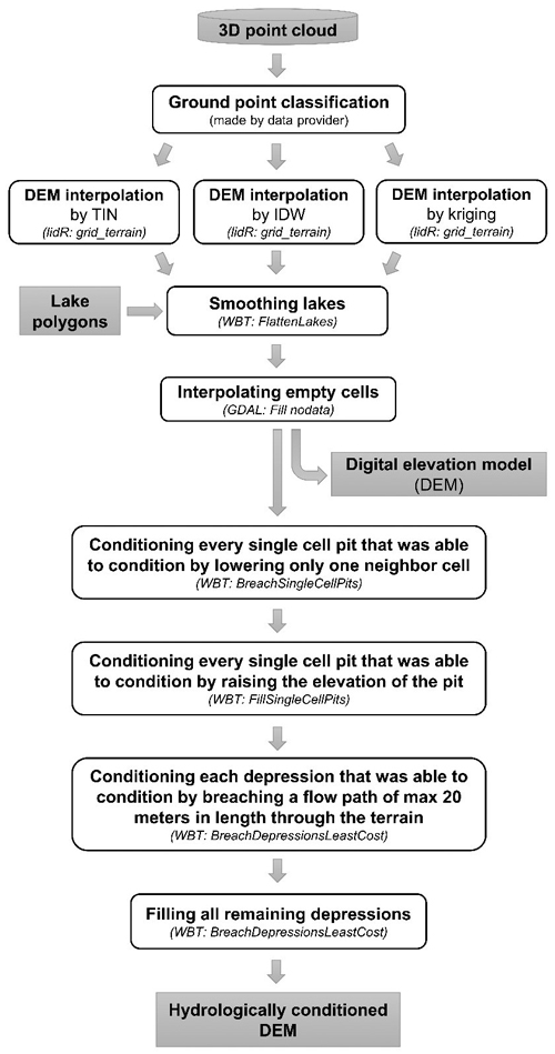
Fig. 2. Workflow of generating a hydrologically conditioned DEM from a LiDAR-derived 3D point cloud. DEM conditioning was an essential part of this study of developing overland flow routing routines by using increased LiDAR data density. Three alternative interpolation methods were tested for DEM processing. The aim is to remove local sinks and depressions that prevent continuous modeling of overland water flow: pits are defined as single cells without any downsloping neighbor and depressions as larger bowl-like features without a downslope direction. Pits and depressions may be artefacts or real, but in any case they need to be either filled or breached for creating a hydrologically conditioned DEM. The open-source tools that were used in the study are named in parenthesis. TIN = Triangulated Irregular Network. IDW = Inverse-distance Weighting. lidR = R package for airborne LiDAR data manipulation and visualization for forestry applications, Version 3.1.2. WBT = WhiteboxTools, Version 1.4.0. GDAL = Geospatial Data Abstraction Library.
The functionality of overland flow routing was tested without any field-inventoried stream/ditch data; thus, water flow paths follow elevation models – not necessarily towards or along ditch network. DEM conditioning was implemented using a stepwise breaching-filling workflow beginning from single cell pits to larger depressions, as suggested by Lindsay (2016), but optimizing the locations for breach paths using the least cost auxiliary topography method proposed by Schwanghart and Kuhn (2010) and recommended by Lidberg et al. (2017). The BreachDepressionsLeastCost tool (Lindsay and Dhun 2015) of the WBT software finds all depressions and identifies possible breach channels that could be carved through dam-like terrain structures. The maximum search distance was set to 20 meters, which was long enough for finding all channels through the widest main road of the study area. The depressions that remained unconditioned after the breaching step were then filled.
When the hydrologically conditioned DEMs were achieved, subsequent stream networks were computed using the D8FlowAccumulation (O’Callaghan and Mark 1984) and ExtractStreams tools of WBT. Four threshold areas were used for defining the minimum area required to initiate and maintain a flow channel: 0.1, 0.2, 0.5, and 1.0 ha. The functionality of differently produced DEMs was compared by calculating the overlapping area of the extracted streams and the streams existing in the topological database of Finland, which is the best widely available ground reference of stream/ditch network with quality based in international standards on map accuracy (Jakobsson 2002; NLS 2021b). In addition, total 40 essential flow routes, 20 culverts, and 20 ditches were manually selected from the study area to investigate how many of these flow paths were correctly detected from different DEM versions.
Wetness indices were produced by first processing the MdInfFlowAccumulation tool (Seibert and McGlynn 2007) of WBT and choosing the output as a specific catchment area (SCA; Gallant and Hutchinson 2011). Also, the TWI was calculated using the WBT software tool WetnessIndex. Comparative TWI indices were examined pairwise by calculating the difference of two raster layers with the same cell size. A kriging-derived wetness index was set as a reference level for the comparisons due to the first results of this study and the support from earlier comparable studies (Chu et al. 2014).
3 Results
Altogether 12 DEM versions were derived based on two point densities, two raster cell sizes, and three interpolation methods (Table 1). Statistics of the DEM conditioning indicates the stepwise breaching-filling technique worked better with high-density LiDAR, as more depressions were conditioned by breaching instead of filling. As the average vertical changes show, an elevation model needs significantly less manipulation when a breach path can be found instead of filling depressions.
| Table 1. Comparison of LiDAR data point densities, DEM cell sizes, and interpolation methods in overland flow routing, which are the main results of this study aiming at improved stream extraction and soil wetness mapping within a forested catchment. In general, breaching leads to more realistic flow paths than filling, and the changes in DEM are smaller on average with breaching. The more overlapping stream/ditch segments were found in the stream extraction, the better flow routing corresponds to the topographical database maintained by the NLS (2021b). However, raster cell may affect flow accumulation, thus the overlaps should not be compared with different cell sizes. Key flow paths were selected so that they were located along the main waterways and were divided roughly evenly within the catchment. | ||||||||||||
| Low-density airborne LiDAR | High-density airborne LiDAR | |||||||||||
| DEM cell size | 1 m | 2 m | 1 m | 2 m | ||||||||
| Interpolation method | TIN | IDW | Kriging | TIN | IDW | Kriging | TIN | IDW | Kriging | TIN | IDW | Kriging |
| Share of remodeled raster cells in conditioned DEM: | ||||||||||||
| Breached cells (>10 cm) | 1.4% | 1.1% | 1.1% | 4.6% | 3.1% | 4.5% | 3.9 % | 3.1% | 3.9% | 6.3% | 5.8% | 6.6% |
| Mean breach depth [m] | –0.18 | –0.11 | –0.12 | –0.14 | –0.13 | –0.14 | –0.12 | –0.11 | –0.12 | –0.16 | –0.16 | –0.17 |
| Filled cells (>10 cm) | 6.0% | 5.9% | 4.9% | 5.8% | 5.6% | 5.1% | 3.4% | 5.6% | 2.8% | 6.4% | 5.6% | 4.0% |
| Mean filling height [m] | 0.62 | 0.51 | 0.43 | 0.45 | 0.48 | 0.37 | 0.53 | 0.46 | 0.44 | 0.52 | 0.55 | 0.35 |
| Overlapped streams/ditches using different channelization thresholds: | ||||||||||||
| 0.1 ha | 73% | 73% | 74% | 70% | 70% | 71% | 76% | 76% | 76% | 72% | 72% | 72% |
| 0.2 ha | 63% | 63% | 64% | 61% | 61% | 62% | 67% | 67% | 67% | 63% | 64% | 64% |
| 0.5 ha | 49% | 50% | 50% | 48% | 48% | 49% | 52% | 53% | 53% | 50% | 50% | 50% |
| 1.0 ha | 38% | 39% | 38% | 37% | 37% | 38% | 39% | 40% | 40% | 38% | 38% | 38% |
| Key flow paths found: | ||||||||||||
| Culverts (n = 20) | 75% | 70% | 75% | 60% | 55% | 60% | 75% | 85% | 85% | 65% | 80% | 85% |
| Streams/ditches (n = 20) | 65% | 55% | 80% | 55% | 70% | 55% | 70% | 85% | 85% | 80% | 90% | 85% |
| Altogether (n = 40) | 70% | 63% | 78% | 58% | 63% | 58% | 73% | 85% | 85% | 73% | 85% | 85% |
The overlap with a digitized stream network was slightly increased with high-density LiDAR, but strict conclusions should not be drawn from the small differences in these percentages. However, the differences were more clear and more affected by interpolation methods when the detection performance was compared in 40 selected flow routes. Both IDW and kriging outperformed TIN algorithm in overland flow routing when high-density LiDAR data were used. However, the choice of DEM cell size did not greatly affect the performance of identification of water channel, brook, or stream locations. A demonstration of mapped flow routes by interpolation and LiDAR point density are shown in Supplementary files S1 and S2.
Pairwise comparison of TWI indices (Fig. 3) shows the same observation as the previous table, i.e., the interpolation method has a smaller effect on overland flow routing than LiDAR point density. TWI indices that were calculated using the same data but different interpolation differ much less from each other than TWI indices derived from the same interpolation (kriging) but different point densities.
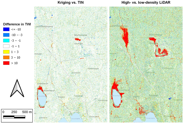
Fig. 3. Comparing the effect of interpolation method (kriging vs. TIN) and LiDAR point density (high vs. low) on Topographic Wetness Index (TWI), which was derived using improved overland flow routing routines developed in this research article. On the left, the difference between TWIs calculated from kriging- and TIN-based elevation models (high-density LiDAR in common). On the right, the respective comparison between high- and low-density LiDAR-derived TWIs (kriging in common). The color scale and symbology are the same in both figures. TWI index was clearly more sensitive to data point density than to interpolation method. Red areas on the right illustrate areas were the TWI computed from low-density LiDAR data was more than 10 units larger than the TWI computed from high-density LiDAR data. For example, the difference is very clear on a mire in the top left, as ditches were poorly recognized by low-density LiDAR, and the whole mire was filled in the DEM conditioning so that continuous flow routing was achieved.
4 Discussion
As assumed, increased LiDAR point density improved overland flow routing due to increased detection of terrain structures. As earlier studies have indicated, kriging is a reliable DEM interpolation method in overland flow routing but IDW worked equally well in this study area. Further studies are needed for comparing kriging and IDW, although some experimental comparisons are available in Zimmermann et al. (1999). However, kriging-algorithm is very heavy and time-consuming compared to IDW, which makes the faster IDW an interesting option in large areas.
Raster cells are key elements of elevation models, and the resolution itself can affect flow accumulation (Ariza-Villaverde et al. 2015). The performance of different cell sizes can be compared in the selected flow paths, which shows that in this study cell size options did not matter when high-density LiDAR data were applied. The larger cell size may be preferred in practical use, as all the processing times are four times quicker when the DEM cell size is doubled.
A higher LiDAR point density significantly improves the accuracy of forest measurements in stand-level forest inventory when point density is less than 1 m–2, but the improvement is moderate with higher pulse densities (Jakubowski et al. 2013). The increased point density enables single-tree forest inventory (Hu et al. 2014), which may promote precision forestry applications, i.e. land manager decision-making at detailed spatial scales (Holopainen et al. 2014; Melander 2021). However, a point density underneath forest canopy can be much lower than 5 m–2 on terrain level, which may influence on flow routing under dense vegetation. In any case, this study can promote further precision forestry-related applications such as dynamic terrain trafficability prediction (Salmivaara et al. 2020), spatially dynamic forest resource planning and management (Mönkkönen et al. 2014), more detailed ditch maintenance planning in peatlands (Laurén et al. 2021), and carbon-optimized landscape management (Holmberg et al. 2021). From global perspective this research offers useful tools for mapping headwater streams and man-made ditches (Ågren and Lidberg 2019).
In future, more programming is needed to improve water flow modeling in drained peatlands. As the ground water table is curvature between two parallel ditches (Laurén et al. 2021), in practice, water flows towards ditches and not necessarily downslope on relatively flat areas. However, current flow routing algorithms allow flow routing only downslope, but new machine learning techniques could enable both the detection of ditch network and consideration of ground water table in flow routing.
5 Conclusions
DEM-derived channel network is needed, for example, in watershed delineation, hydrological modeling, and natural resource management at detailed spatial scales. In a forested area, overland flow routing can be improved with high-density airborne LiDAR data. The TIN method has commonly been used in DEM interpolation, but this research clearly suggests that more sophisticated interpolation methods, such as kriging or IDW, unless they are computationally more time-demanding than TIN, should be applied for achieving all the benefits that high-density LiDAR data can offer. However, from this viewpoint, no reasons were found to decrease the DEM raster cell size from 2 meters, which is used, for example, in the Finnish nationwide elevation model.
The whole area of Finland will be covered by high-density LiDAR data within six years, so this study contributes to a topical question of finding additional value and new practices for adapting these data in environmental modeling. As all the algorithms used in the study are available from open-source software, the utilization of LiDAR data is cost-effective for both science and business. As high-density LiDAR data are becoming extensively available in following years, it is useful to investigate what possibilities the data of new standards can give for forest resource management.
Declaration of openness of research materials, data, and code
The low-density LiDAR data and the topographic database are freely available in the open data file service of NLS Finland (https://www.maanmittauslaitos.fi/en/e-services/open-data-file-download-service). Access to the full-density LiDAR data is licensed and charged, and more information is available here: https://www.maanmittauslaitos.fi/en/maps-and-spatial-data/expert-users/product-descriptions/laser-scanning-data-5-p.
Authors’ contributions
Mikko Niemi defined the research design, implemented the analysis, and wrote the scientific report.
Acknowledgements
I want to thank my supervisor, professor Jari Vauhkonen from the University of Helsinki, for his valuable comments and suggestions on the manuscript, the analysis, and the interpretation of results, as well as his professional guidance and unselfish support in my dissertation project. I’m also thankful for Anne Mäkynen from the Centre for Economic Development, Transport and the Environment (ELY Centre), who proposed a suitable study area from the Pirkanmaa region. Also, warm thanks to Antti Leinonen and Mikko Kesälä from the Finnish Forest Centre for interesting discussions on the topic, and useful hints on the WhiteboxTools software.
Funding
This work was supported by the Academy of Finland (grant number 324193), and by the University of Helsinki. In addition, the ELY Centre of Pirkanmaa paid the license of high-density airborne LiDAR data from the Parkano area.
References
Ågren AM, Lidberg W (2019) The importance of better mapping of stream networks using high resolution digital elevation models – upscaling from watershed scale to regional and national scales. Hydrol Earth Syst Sci Discuss. [preprint]. https://doi.org/10.5194/hess-2019-34.
Ågren AM, Lidberg W, Strömgren M, Ogilvie J, Arp PA (2014) Evaluating digital terrain indices for soil wetness mapping – a Swedish case study. Hydrol Earth Syst Sci 18: 3623–3634. https://doi.org/10.5194/hess-18-3623-2014.
Ariza-Villaverde AB, Jiménez-Hornero FJ, Gutiérrez de Ravé E (2015) Influence of DEM resolution on drainage network extraction: a multifractal analysis. Geomorphology 241: 243–254. https://doi.org/10.1016/j.geomorph.2015.03.040.
Arun PV (2013) A comparative analysis of different DEM interpolation methods. Egypt J Rem Sens 16: 133–139. https://doi.org/10.1016/j.ejrs.2013.09.001.
Callow JN, van Niel KP, Boggs GS (2007) How does modifying a DEM to reflect known hydrology affect subsequent terrain analysis? J Hydrol 332: 30–39. https://doi.org/10.1016/j.jhydrol.2006.06.020.
Chu H-J, Wang C-K, Huang M-L, Lee C-C, Liu CY, Lin C-C (2014) Effect of point density and interpolation of LiDAR-derived high-resolution DEMs on landscape scarp identification. Gisci Remote Sens 51: 731–747. https://doi.org/10.1080/15481603.2014.980086.
Duke GD, Kienzle SW, Johnson DL, Byrne JM (2006) Incorporating ancillary data to refine anthropogenically modified overland flow paths. Hydrol Process 20: 1827–1843. https://doi.org/10.1002/hyp.5964.
Frizzle C, Fournier RA, Trudel M, Luther JE (2021) Using the Soil and Water Assessment Tool to develop a LiDAR-based index of the erosion regulation ecosystem service. J Hydrol 595, article id 126009. https://doi.org/10.1016/j.jhydrol.2021.126009.
Gallant JC, Hutchinson MF (2011) A differential equation for specific catchment area. Water Resour Res 47, article id W05535. https://doi.org/10.1029/2009WR008540.
Guo Q, Li W, Yu H, Alvarez O (2010) Effects of topographic variability and lidar sampling density on several dem interpolation methods. Photogramm Eng Rem S 6: 701–712. https://doi.org/10.14358/PERS.76.6.701.
Heritage GL, Milan DJ, Large ARG, Fuller IC (2009) Influence of survey strategy and interpolation model on DEM quality. Geomorphology 112: 334–344. https://doi.org/10.1016/j.geomorph.2009.06.024.
Holopainen M, Vastaranta M, Hyyppä J (2014) Outlook for the next generation’s precision forestry in Finland. Forests 5: 1682–1694. https://doi.org/10.3390/f5071682.
Holmberg M, Akujärvi A, Anttila S, Autio I, Haakana M, Junttila V, Karvosenoja N, Kortelainen P, Mäkelä A, Minkkinen K, Minunho F, Rankinen K, Ojanen P, Paunu V-V, Peltoniemi M, Rasilo T, Sallantaus T, Savolahti M, Tuominen Sa, Tuominen Se, Vanhala P, Forsius M (2021) Sources and sinks of greenhouse gases in the landscape: approach for spatially explicit estimates. Sci Total Environ 781, article 146668. https://doi.org/10.1016/j.scitotenv.2021.146668.
Holmgren P (1994) Multiple flow direction algorithms for runoff modelling in grid based elevation models: an empirical evaluation. Hydrol Process 8: 327–334. https://doi.org/10.1002/hyp.3360080405.
Hu B, Li J, Jing L, Judah A (2014) Improving the efficiency and accuracy of individual tree crown delineation from high-density LiDAR data. Int J Appl Earth Obs 26: 145–155. https://doi.org/10.1016/j.jag.2013.06.003.
Jaboyedoff M, Oppikofer T, Abellán A, Derron M-H, Loye A, Metzger R, Pedrazzini A (2012) Use of LIDAR in landslide investigations: a review. Nat Hazards 61: 5–28. https://doi.org/10.1007/s11069-010-9634-2.
Jakobsson A (2002) Data quality and quality management – examples of quality evaluation procedures and quality management in European National Mapping Agencies. In: Wenzhong S, Fisher P, Goodchild MF (eds) Spatial data quality. Taylor & Francis, London, pp 216–229. https://doi.org/10.1201/b12657.
Jakubowski MK, Guo Q, Kelly M (2013) Tradeoffs between lidar pulse density and forest measurement accuracy. Remote Sens Environ 130: 245–253. https://doi.org/10.1016/j.rse.2012.11.024.
Jenson SK, Domingue JO (1988) Extracting topographic structure from digital elevation data for geographic information system analysis. Photogramm Eng Rem S 54: 1593–1600.
Kanostrevac D, Borisov M, Bugarinovic Z, Ristic A, Radulovic A (2019) Data quality comparative analysis of photogrammetric and Lidar DEM. Micro Macro Mezzo Geo Inf 12: 17–34.
Kraus K, Pfeifer N (1998) Determination of terrain models in wooded areas with airborne laser scanner data. ISPRS J Photogramm 53: 193–203. https://doi.org/10.1016/S0924-2716(98)00009-4.
Launiainen S, Guan M, Salmivaara A, Kieloaho A-J (2019) Modeling boreal forest evapotranspiration and water balance at stand and catchment scales: a spatial approach. Hydrol Earth Syst Sci 23: 3457–3480. https://doi.org/10.5194/hess-23-3457-2019.
Laurén A, Palviainen M, Launiainen S, Leppä K, Stenberg L, Urzainki I, Nieminen M, Laiho R, Hökkä H (2021) Drainage and stand growth response in peatland forests – description, testing, and application of mechanistic peatland simulator SUSI. Forests 12, article id 293. https://doi.org/10.3390/f12030293.
Lidberg W, Nilsson M, Lundmark T, Ågren AM (2017) Evaluating preprocessing methods of digital elevation models for hydrological modelling. Hydrol Process 31: 4660–4668. https://doi.org/10.1002/hyp.11385.
Lidberg W, Nilsson M, Ågren A (2020) Using machine learning to generate high-resolution wet area maps for planning forest management: a study in a boreal forest landscape. Ambio 49: 475–486. https://doi.org/10.1007/s13280-019-01196-9.
Lindsay JB (2016) Efficient hybrid breaching-filling sink removal methods for flow path enforcement in digital elevation models. Hydrol Process 30: 846–857. https://doi.org/10.1002/hyp.10648.
Lindsay JB (2020) WhiteboxTools User Manual, Version 1.4.0. https://jblindsay.github.io/wbt_book/preface.html. Accessed 22 April 2020.
Lindsay JB, Creed IF (2005) Removal of artifact depressions from digital elevation models: towards a minimum impact approach. Hydrol Process 19: 3113–3126. https://doi.org/10.1002/hyp.5835.
Lindsay JB, Dhun K (2015) Modelling surface drainage patterns in altered landscapes using LiDAR. Int J Geogr Inf Sci 29: 397–411. https://doi.org/10.1080/13658816.2014.975715.
Maguya AS (2015) Use of airborne laser scanning data in demanding forest conditions. Acta Universitatis Lappeenrantaensis 683. http://urn.fi/URN:ISBN:978-952-265-903-3.
Maltamo M, Naesset E, Vauhkonen J (2014) Forestry Applications of Airborne Laser Scanning. Managing Forest Ecosystems 27. Springer Netherlands. https://doi.org/10.1007/978-94-017-8663-8.
Martz LW, Garbrecht J (1998) The treatment of flat areas and depressions in automated drainage analysis of raster digital elevation models. Hydrol Process 12: 843–855. https://doi.org/10.1002/(SICI)1099-1085(199805)12:6%3C843::AID-HYP658%3E3.0.CO;2-R.
Martz LW, Garbrecht J (1999) An outlet breaching algorithm for the treatment of closed depressions in a raster DEM. Comput Geosci 25: 835–844. https://doi.org/10.1016/S0098-3004(99)00018-7.
Melander L (2021) Towards precision forestry: methods for environmental perception and data fusion in forest operations. Tampere University Dissertations 379. http://urn.fi/URN:ISBN:978-952-03-1863-5.
Mohamedou C, Tokola T, Eerikäinen K (2017) LiDAR-based TWI and terrain attributes in improving parametric predictor for tree growth in southeast Finland. Int J Appl Earth Obs 62: 183–191. https://doi.org/10.1016/j.jag.2017.06.004.
Mönkkönen M, Juutinen A, Mazziotta A, Miettinen K, Podkopaev D, Reunanen P, Salminen H, Tikkanen O-P (2014) Spatially dynamic forest management to sustain biodiversity and economic returns. J Environ Manage 134: 80–89. https://doi.org/10.1016/j.jenvman.2013.12.021.
Muhadi NA, Abdullah AF, Bejo SK, Mahadi MR, Mijic A (2020) The use of LiDAR-derived DEM in flood applications: a review. Remote Sens 12, article id 2308. https://doi.org/10.3390/rs12142308.
Murphy PNC, Ogilvie J, Connor K, Arp PA (2007) Mapping wetlands: a comparison of two different approaches for New Brunswick, Canada. Wetlands 27: 846–854. https://doi.org/10.1672/0277-5212(2007)27[846:MWACOT]2.0.CO;2.
Murphy PNC, Ogilvie J, Meng F-R, Arp P (2008) Stream network modelling using lidar and photogrammetric digital elevation models: a comparison and field verification. Hydrol Process 22: 1747–1754. https://doi.org/10.1002/hyp.6770.
Murphy PNC, Ogilvie J, Arp P (2009) Topographic modelling of soil moisture conditions: a comparison and verification of two models. Eur J Soil Sci 60: 94–109. https://doi.org/10.1111/j.1365-2389.2008.01094.x.
National Land Survey of Finland (NLS) (2021a) Laser scanning data 5 p. https://www.maanmittauslaitos.fi/en/maps-and-spatial-data/expert-users/product-descriptions/laser-scanning-data-5-p. Accessed 1 October 2021.
National Land Survey of Finland (NLS) (2021b) Topographic database. https://www.maanmittauslaitos.fi/en/maps-and-spatial-data/expert-users/product-descriptions/topographic-database. Accessed 13 October 2021.
Niemi MT, Vastaranta M, Vauhkonen J, Melkas T, Holopainen M (2017) Airborne LiDAR-derived elevation data in terrain trafficability mapping. Scand J Forest Res 32: 762–773. https://doi.org/10.1080/02827581.2017.1296181.
O’Callaghan JF, Mark DM (1984) The extraction of drainage networks from digital elevation data. Comput Vision Graph 28: 323–344. https://doi.org/10.1016/S0734-189X(84)80011-0.
Pei T, Qin C-Z, Zhu A-X, Yang L, Luo M, Li B, Zhou C (2010). Mapping soil organic matter using the topographic wetness index: a comparative study based on different flow-direction algorithm and kriging methods. Ecol Indic 10: 610–619. https://doi.org/10.1016/j.ecolind.2009.10.005.
Roussel J-R, Auty D, Coops NC, Tompalski P, Goodbody TRH, Sánchez Meador A, Bourdon J-F, de Boissieu F, Achim A (2020) lidR: an R package for analysis of Airborne Laser Scanning (ALS) data. Remote Sens Environ 251, article id 112061. https://doi.org/10.1016/j.rse.2020.112061.
Quinn P, Beven K, Chevallier P, Planchon O (1991) The prediction of hillslope flow paths for distributed hydrological modelling using digital terrain models. Hydrol Process 5: 59–79. https://doi.org/10.1002/hyp.3360050106.
Salmivaara A, Launiainen S, Perttunen J, Nevalainen P, Pohjankukka J, Ala-Ilomäki J, Sirén M, Laurén A, Tuominen S, Uusitalo J, Pahikkala T, Heikkonen J, Finér L (2020) Towards dynamic forest trafficability prediction using open spatial data, hydrological modelling and sensor technology. Forestry 93: 662–674. https://doi.org/10.1093/forestry/cpaa010.
Schwanghart W, Kuhn NJ (2010) TopoToolbox: a set of Matlab functions for topographic analysis. Environ Model Softw 25: 770–781. https://doi.org/10.1016/j.envsoft.2009.12.002.
Seibert J, McGlynn BL (2007) A new triangular multiple flow direction algorithm for computing upslope areas from gridded digital elevation models. Water Resour Res 43, article id W04501. https://doi.org/10.1029/2006WR005128.
Sharma M, Garg RD, Badenko V, Fedotov A, Min L, Yao A (2020) Potential of airborne LiDAR data for terrain parameters extraction. Quatern Int 575–576: 317–327. https://doi.org/10.1016/j.quaint.2020.07.039.
Tarboton DG (1997) A new method for the determination of flow directions and upslope areas in grid digital elevation models. Water Resour Res 33: 309–319. https://doi.org/10.1029/96WR03137.
Vosselman G (2000) Slope based filtering of laser altimetry data. IAPRS 33: 935–942.
Wang L, Liu H (2006) An efficient method for identifying and filling surface depressions in digital elevation models for hydrologic analysis and modelling. Int J Geogr Inf Sci 20: 193–213. https://doi.org/10.1080/13658810500433453.
Wilson JP, Aggett G, Yongxin D, Lam CS (2008) Water in the landscape: a review of contemporary flow routing algorithms. In: Zhou Q, Lees B, Tang G (eds) Advances in digital terrain analysis. Lecture Notes in Geoinformation and Cartography. Springer, Berlin, Heidelberg, pp 213–236. https://doi.org/10.1007/978-3-540-77800-4_12.
Woodrow K, Lindsay JB, Berg AA (2016) Evaluating DEM conditioning techniques, elevation source data, and grid resolution for field-scale hydrological parameter extraction. J Hydrol 540: 1022–1029. https://doi.org/10.1016/j.jhydrol.2016.07.018.
Zimmerman D, Pavlik C, Ruggles A, Armstrong MP (1999) An experimental comparison of ordinary and universal kriging and inverse distance weighting. Math Geol 31: 375–390. https://doi.org/10.1023/A:1007586507433.
Total of 57 references.
