Timo Pukkala,
Kjersti Holt Hanssen  ,
Kjell Andreassen
,
Kjell Andreassen
Stem taper and bark functions for Norway spruce in Norway
Pukkala T., Holt Hanssen K., Andreassen K. (2019). Stem taper and bark functions for Norway spruce in Norway. Silva Fennica vol. 53 no. 3 article id 10187. https://doi.org/10.14214/sf.10187
Highlights
- New variable-exponent stem taper and bark functions were developed for Norway spruce
- Both fixed and mixed-effects models were developed
- Site index and tree age had statistically significant but small effects on stem taper.
Abstract
Based on data from long-term experimental fields with Norway spruce (Picea abies (L.) H. Karst.), we developed new stem taper and bark functions for Norway. Data was collected from 477 trees in stands across Norway. Three candidate functions which have shown good performance in previous studies (Kozak 02, Kozak 97 and Bi) were fitted to the data as fixed-effects models. The function with the smallest Akaike Information Criterion (AIC) was then chosen for additional analyses, fitting 1) site index-dependent and 2) age-dependent versions of the model, and 3) fitting a mixed-effects model with tree-specific random parameters. Kozak 97 was found to be the function with the smallest AIC, but all three tested taper functions resulted in fairly similar predictions of stem taper. The site index-dependent function reduced AIC and residual standard error and showed that the effect of site index on stem taper is different in small and large trees. The predictions of the age-independent and age-dependent models were very close to each other. Adding tree-specific random parameters to the model clearly reduced AIC and residual variation. However, the results suggest that the mixed-effects model should be used only when it is possible to calibrate it for each tree, otherwise the fixed-effects Kozak 97 model should be used. A model for double bark thickness was also fitted as fixed-effects Kozak 97 model. The model behaved logically, predicting larger relative but smaller absolute bark thickness for small trees.
Keywords
forest management;
Picea abies;
Kozak model;
variable-exponent taper function
-
Pukkala,
University of Eastern Finland, P.O. Box 111, FI-80101 Joensuu, Finland
 https://orcid.org/0000-0003-2853-9510
E-mail
timo.pukkala@uef.fi
https://orcid.org/0000-0003-2853-9510
E-mail
timo.pukkala@uef.fi
-
Holt Hanssen,
Norwegian Institute of Bioeconomy Research, P.O. Box 115, NO-1431 Ås, Norway
https://orcid.org/0000-0002-1715-3092
E-mail
kjersti.hanssen@nibio.no
-
Andreassen,
Norwegian Institute of Bioeconomy Research, P.O. Box 115, NO-1431 Ås, Norway
https://orcid.org/0000-0003-4272-3744
E-mail
kjell.andreassen@nibio.no
Received 30 April 2019 Accepted 10 September 2019 Published 16 September 2019
Views 51068
Available at https://doi.org/10.14214/sf.10187 | Download PDF

1 Introduction
Taper models predict diameter at any location along the stem of a tree. Such functions are used to estimate the total timber volume and assortment volumes of trees. They are essential tools in forest growth and yield models, as well as in forest inventory and management planning systems (Kozak 2004; Kublin et al. 2013). They are also needed in various simulation models, e.g. for simulating the spread of root and butt rot (Heterobasidion ssp.) in Norway spruce (Picea abies (L.) H. Karst.) stands (Pukkala et al. 2005).
Many forms and types of taper models have been reported and evaluated during the past decades (Sterba 1980; Kozak 2004). The models can be classified into single, segmented and variable-exponent models (Rojo et al. 2005). Tree trunks vary in form from bottom to top, with a neiloid form at the bottom followed by a paraboloid in the middle and a cone shape at the top, and several intermediate forms along the stem. Simple parametric models usually fail to account for this change in geometry. To deal with this challenge, splines may be used to approximate the stem form in cases where several diameters along the stem are known.
Variable-exponent taper functions were introduced in the eighties (Kozak 1988; Newnham 1988) and they consist of an exponential mean function whose exponent is changing along the trunk to describe different geometrical shapes from stump to top (Kublin et al. 2013). Examples include Muhairwe et al. (1994), Kozak (1997) and Bi (2000). Kozak (2004) tested four variable-exponent functions on several tree species and biogeoclimatic zones, and concluded that his model “02” consistently performed best for estimating stem diameter inside bark, tree or log volumes, and merchantable height.
Most taper functions use diameter at breast height (dbh) and total tree height as predictor variables. In addition, stand variables like tree density, basal area or site index are likely to affect stem form. However, using stand variables to predict stem taper may be problematic in simulations. If for instance a thinning is simulated, basal area, mean diameter and other stand variables will change and, consequently, predicted stem profiles of the trees will also change, although they are exactly the same trees before and after thinning. Nevertheless, factors like site index or tree age can be included in taper functions, as they do not change instantly due to thinning.
In Norway, up till now the taper tables by Eide and Langsæter (1929) and their extended version by Eide and Langsæter (1954) have been used for diameter predictions in Norway spruce. Gjølberg (1978) developed a set of functions based on some of the material from Eide and Langsæter’s tables. These functions predict stem diameter at certain relative heights. Interpolation is need for calculating diameters at other heights. Since these functions are old and predict the stem diameter only for a small number of relative heights, there is a need for updated and more modern types of taper functions. Based on data from long-term experimental fields with Norway spruce, we have developed new stem taper and bark functions for Norway.
2 Material and methods
2.1 Data material and measurements
The data set included 477 Norway spruce trees from 14 counties in Norway (Table 1). A total of 39 sites belonging to NIBIO’s (Norwegian Institute of Bioeconomy Research) long-term field trials were selected to cover a range of site indices, tree sizes, stand ages and regions in Norway. Most counties in Norway where Norway spruce occurs naturally are represented. The shape of the plots was mostly rectangular or square and the mean plot area was 1675 m2.
| Table 1. Site index (H40, Tveite 1977) and characteristics of the taper sample trees. Mean values of diameter and height for sample trees within each site, with min-max in parenthesis. Diameter and bark thickness at breast height. Crown height up to the lowest green branch whorl. | |||||||
| Site no. | Site index (H40, m) | No. of taper trees | D (cm) | H (m) | Double bark (mm) | Crown height (m) | County |
| 25 | 21 | 15 | 27 (6–55) | 23 (7–34) | 14 | 11 | Akershus |
| 33 | 12 | 15 | 16 (7–26) | 16 (9–23) | 11 | 11 | Akershus |
| 37 | 12 | 15 | 23 (11–41) | 17 (10–24) | 17 | 9 | Nord-Trøndelag |
| 39 | 7 | 16 | 15 (7–24) | 13 (7–17) | 12 | 8 | Nord-Trøndelag |
| 42 | 20 | 15 | 23 (7–34) | 20 (9–25) | 11 | 15 | Akershus |
| 62 | 14 | 15 | 16 (10–32) | 15 (10–20) | 12 | 8 | Nordland |
| V70 | 24 | 2 | 81 (70–92) | 42 (41–43) | 27 | 23 | Hordaland |
| 91 | 23 | 16 | 14 (6–24) | 15 (7–22) | 8 | 7 | Akershus |
| 139 | 16 | 16 | 12 (4–21) | 10 (4–17) | 9 | 4 | Oppland |
| 143 | 12 | 15 | 23 (11–39) | 17 (10–24 | 18 | 8 | Nord-Trøndelag |
| 158 | 16 | 15 | 12 (3–20) | 11 (3–18) | 12 | 7 | Oppland |
| 162 | 19 | 15 | 24 (8–40) | 21 (8–27) | 16 | 12 | Oppland |
| 164 | 14 | 15 | 34 (20–51) | 26 (20–30) | 19 | 13 | Oppland |
| 168 | 23 | 15 | 11 (3–16) | 12 (4–19) | 6 | 8 | Østfold |
| 174 | 21 | 15 | 19 (4–34) | 13 (5–19) | 11 | 8 | Østfold |
| 176 | 20 | 15 | 23 (5–45) | 19 (4–27) | 12 | 12 | Oslo |
| 210 | 11 | 15 | 26 (7–44) | 18 (8–23) | 18 | 10 | Nord-Trøndelag |
| 214 | 18 | 17 | 18 (6–29) | 15 (6–23) | 9 | 9 | Sør-Trøndelag |
| 219 | 15 | 16 | 21 (5–34) | 19 (4–24) | 14 | 12 | Hedmark |
| 223 | 16 | 15 | 20 (7–39) | 17 (6–24) | 12 | 9 | Hedmark |
| 228 | 21 | 15 | 13 (10–18) | 13 (11–17) | 8 | 7 | Oslo |
| 237 | 15 | 2 | 45 (42–48) | 27 (26–28) | 21 | 10 | Sør-Trøndelag |
| 239 | 18 | 15 | 24 (10–48) | 20 (10–26) | 15 | 10 | Sør-Trøndelag |
| 252 | 16 | 5 | 41 (31–53) | 23 (18–25) | 22 | 5 | Oppland |
| 253 | 14 | 5 | 18 (11–28) | 13 (7–21) | 12 | 5 | Oppland |
| 254 | 15 | 5 | 20 (11–42) | 13 (8–22) | 13 | 8 | Oppland |
| 262 | 21 | 15 | 19 (11–35) | 18 (11–26) | 10 | 10 | Akershus |
| 348 | 15 | 1 | 12 (12–12) | 13 (13–13) | 25 | 3 | Aust-Agder |
| 377 | 13 | 11 | 18 (12–25) | 17 (11–22) | 15 | 11 | Buskerud |
| 402 | 21 | 15 | 22 (10–36) | 20 (11–26) | 12 | 10 | Vestfold |
| 406 | 22 | 15 | 18 (11–23) | 20 (13–24) | 10 | 14 | Vestfold |
| 452 | 13 | 15 | 12 (41–6) | 10 (3–14) | 9 | 4 | Nord-Trøndelag |
| 459 | 25 | 15 | 25 (12–39) | 23 (16–27) | 10 | 14 | Telemark |
| 512 | 15 | 5 | 16 (12–15) | 14 (12–15) | 11 | 9 | Oslo |
| 514 | 11 | 7 | 10 (4–14) | 10 (4–15) | 8 | 4 | Hedmark |
| 519 | 20 | 4 | 12 (10–15) | 13 (9–16) | 9 | 7 | Hedmark |
| 540 | 19 | 4 | 11 (10–14) | 9 (8–11) | 7 | 2 | Østfold |
| 593 | 15 | 15 | 16 (8–23) | 14 (9–20) | 9 | 5 | Troms |
| 611 | 16 | 15 | 11 (3–21) | 10 (3–16) | 6 | 4 | Nordland |
| D = diameter at breast height; H = tree height from ground to top | |||||||
In accordance with NIBIOs instructions for long-term field trials (e.g. Braastad 1980), every fifth tree along the tree numbers of the respective plot was selected as a sample tree for additional measurements (tree height, crown height and in some cases tree age) in addition to breast height diameter. Thus, the whole diameter distribution of the stand was represented. The sample trees were used to describe the stand. Subsequently, taper trees were subjectively selected from these sample trees to represent a broad range of the diameter distribution and different within-plot locations. The selected taper trees represented most of the 2-cm diameter classes although higher priority was given to the largest diameter classes. Each taper tree was felled before the measurements took place. On average, 12 trees per plot were measured for stem taper.
The measurements took place at different occasions so that different tree ages and stand characteristics, from young stands up to the end of the rotation, were represented. Most plots were visited for taper measurements several times, the longest interval between the first and last taper measurement in the same plot being 51 years. In some plots, however, taper trees were measured only in one year. A few trees older than normal rotation age were also measured. The data collection took place over an extended period, from 1920 to 2016.
The trees were felled before measurement, and the total height was determined from the felled tree. For each one-meter section of the stem, diameter over bark was measured crosswise with a calliper, and bark thickness was also measured with a bark gauge from both sides of the tree. The mean value of the two perpendicular diameters as well as the two bark measurements were used in the present study.
2.2 Statistical methods
The taper model was developed along the following steps: First, three candidate functions which have shown good performance in previous studies (Kozak 2004; Heiðarsson and Pukkala 2011; de-Miguel et al. 2012) were compared. These models were the taper functions of Kozak (1997), Kozak (2004) and Bi (2000), henceforth referred to as Kozak 97, Kozak 02 and Bi. Each of these models was fitted to the data as a fixed-effects model, and the function with the smallest AIC (Akaike Information Criterion) was chosen for additional analyses.
The candidate equations were as follows:


where d is diameter (cm) at height h (m), D is dbh (cm), H is total tree height (m), q is h/H, t is 1.3/H, X is (1–q1/3)/(1–t1/3), Y is (1–q1/2)/(1–t1/2) and Q is (1–q1/3).
The additional analyses consisted of fitting site index-dependent and age-dependent versions of the model, and fitting the model as a mixed-effects model. Fitting the site index- and age-dependent models consisted of making all parameters dependent on site index or tree age, which doubled the number of parameters. For example, parameter a0 of Kozak 97 was replaced by (a01+a02SI) where SI is the site index in the Norwegian site classification system (Tveite (1977), dominant height at 40 years, m).
The taper data formed a hierarchical structure where several trees were measured from the same county and plot, and several diameters were measured from the same tree. Diameters measured in the same plot or from the same tree were correlated observations. Consequently, the significance of the parameter estimates of ordinary least squares models are not reliable. These correlations were taken into account in mixed-effects modelling. When fitting mixed-effects models, one or several of the parameters were assumed to be plot- or tree-specific, having a random component for each plot or tree. For example, parameter a0 of Kozak 97 was replaced by (a0+α0i ) where α0i is a random parameter for plot i or tree i. The random effects that were added to different parameters were assumed to follow a multivariate normal distribution.
The mixed-effects models were fitted using the nlme function available in the nlme package of the R software (Pinheiro et al. 2018). Random components were added to different parameters, and the best combination of random parameters was found by trial and error, using the AIC and the residual variation of the full model as the criteria. Random parameters also partly account for the autocorrelation of residuals at different heights along the stem (Arias-Rodil et al. 2015).
The new fixed-effects model was tested against the old taper model by Gjølberg (1978) using visual comparisons of stem profiles from both typical and untypical combinations of dbh and height.
3 Results
3.1 Baseline fixed-effects model
Of the three candidate functions, Kozak 97 resulted in the smallest AIC value, and it was therefore selected as the baseline taper model (Table 2). The AIC values of the three functions were Kozak 97: 22059; Kozak 02: 22205; and Bi: 23164. The residual standard errors were Kozak 97: 0.961; Kozak 02: 0.970; and Bi: 1.03. The three tested taper functions resulted in fairly similar predicted stem taper (Fig. 1). Especially Kozak 97 and Kozak 02 were very close to each other.
| Table 2. Parameters of the fixed-effects Kozak 97 model for stem taper over bark. | ||
| Parameter | Estimate | t value |
| a0 | 0.8795844 | 142.01 |
| a1 | 0.9457765 | 244.79 |
| a2 | 0.1061692 | 20.06 |
| b1 | 0.6624965 | 102.80 |
| b2 | 0.3781478 | 50.36 |
| b3 | –0.4418430 | –21.04 |
| b4 | –0.5154988 | –37.38 |
| b5 | 0.0197963 | 41.52 |
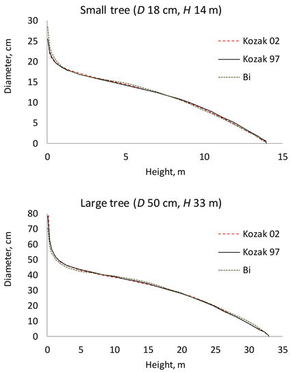
Fig. 1. Stem profiles predicted for a small and a large tree using the three tested taper functions. D is diameter at breast height; H is tree height from ground to top.
3.2 Site index-dependent model
Kozak 97 was further fitted so that all parameters depended on either site index or tree age. Despite a high number of parameters, almost all of them were significant, which means that most parameters were statistically significantly dependent on site index or age (Tables 3 and 4).
| Table 3. Parameters of the site index-dependent fixed-effects Kozak 97 model for stem taper over bark. | ||||
| Parameter | Constant | Slope coefficient | ||
| Estimate | t value | Estimate | t value | |
| a0 | 1.0233871 | 30.14 | –0.0074925 | –4.10 |
| a1 | 1.1012260 | 60.36 | –0.0084932 | –8.80 |
| a2 | –0.1160389 | –4.30 | 0.0119276 | 0.00 |
| b1 | 0.9717245 | 35.10 | –0.0161964 | –11.07 |
| b2 | 0.0787199 | 2.44 | 0.0153552 | 8.91 |
| b3 | –1.4247046 | –15.34 | 0.0488699 | 10.16 |
| b4 | –0.7021483 | –11.21 | 0.0105041 | 3.29 |
| b5 | 0.0486118 | 22.22 | –0.0014326 | –13.30 |
| Table 4. Parameters of the age-dependent fixed-effects Kozak 97 model for stem taper over bark. | ||||
| Parameter | Constant | Slope coefficient | ||
| Estimate | t value | Estimate | t value | |
| a0 | 0.8294 | 44.76 | 0.0006427 | 3.06 |
| a1 | 0.8600 | 69.38 | 0.0008741 | 7.21 |
| a2 | 0.2179 | 13.39 | –0.001193 | –7.13 |
| b1 | 0.5449 | 24.13 | 0.001253 | 5.84 |
| b2 | 0.5581 | 21.74 | –0.001806 | –7.32 |
| b3 | –0.07002 | –0.93 | –0.003486 | –4.68 |
| b4 | –0.4296 | –9.07 | –0.001174 | –2.51 |
| b5 | 9.725e-03 | 4.87 | 8.524e-05 | 4.57 |
By allowing the parameters to change as a function of site index reduced AIC from 22059 to 21670 and residual standard error from 0.961 to 0.937. Fig. 2 shows that site index had a visible effect on stem taper. A small tree growing on a poor site had a slightly more conical stem shape than a small tree growing on more fertile site (when dbh and height were the same). For a large tree, the diameters in the middle part of the stem were smaller on a poor site.
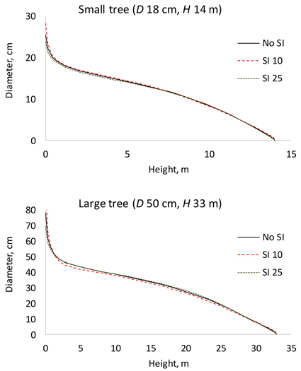
Fig. 2. Effect of site index (SI) on stem taper in a small and a large tree. The continuous line shows the stem taper according to the baseline model (Table 2). D is diameter at breast height; H is tree height from ground to top.
3.3 Age-dependent model
Age was not available for all trees. Therefore, only 6468 diameter observations out of the total 7974 diameter measurements could be used for fitting the age-dependent taper model (Table 4). The AIC of the age-dependent model was 18107 and the residual standard error was 0.976. These values are not directly comparable to those of the baseline model since the age-dependent model was based on a smaller dataset. Although tree age had a significant effect on most parameters of the Kozak 97 model, the predictions of the age-independent and age-dependent models were very close to each other.
3.4 Mixed-effects model
Adding plot-specific random parameters to the baseline model improved the model only very little. The opposite was true for tree-specific parameters, which clearly reduced the AIC and residual variation of the model. The random components of parameters a0, a1, and a2 correlated very strongly with each other, and it was enough to have a random parameter for only one of them. Randomizing up to three of parameters b1 to b5 improved the model clearly. The best model was obtained when parameter b1, b2 and b5 were randomized (Table 5). Therefore, the mixed-effects taper model was as follows:
| Table 5. Parameters of the mixed-effects Kozak 97 model for stem taper over bark. | |||
| Parameter | Fixed effect | Standard deviation of random effect | |
| Estimate | t value | ||
| a0 | 0.9574392 | 115.43 | - |
| a1 | 0.9874995 | 192.41 | 0.006438417 |
| a2 | 0.0313538 | 4.77 | - |
| b1 | 0.6955883 | 53.39 | 0.087608971 |
| b2 | 0.2987029 | 49.33 | 0.079936209 |
| b3 | –0.7959772 | –68.74 | - |
| b4 | –0.3967074 | –11.80 | - |
| b5 | 0.0334238 | 49.34 | 0.009906016 |

where α1i, β1i, β2i and β5i are random effects for tree i. The AIC of the full mixed-effects model was 11129, which is much less than obtained for the corresponding fixed-effects model (22059). The residual standard error decreased from 0.961 to 0.376.
The correlations of the random parameters of the mixed-effects model are given in Table 6.
| Table 6. Correlations of the random parameters of the mixed-effects model. | |||
| α1i | β1i | β2i | |
| β1i | –0.014 | ||
| β2i | 0.172 | –0.423 | |
| β5i | 0.180 | –0.547 | 0.187 |
3.5 Comparison of the models
The results for AIC and residual standard error indicate that the (full) mixed-effects model is by far the most accurate. The same can also be seen from Fig. 3, which shows that the residuals are much smaller for the mixed-effects model than for the other models. However, reaching good performance of the mixed-effects model requires that the random parameters are known, i.e., the model is calibrated for a particular tree (Arias-Rodil et al. 2015). Since this is seldom the case, it makes sense to compare the predictive capacity of the fixed part of the mixed-effects model to that of the other models. When the residual standard error was calculated for the fixed part of the mixed-effects model, assuming that all random parameters are zero, it was 1.076, which is more than obtained for the baseline fixed-effects model (0.961) or the site index-dependent fixed-effects model (0.937). The overall bias (mean prediction errors) was 0.032 cm for the baseline model (0.32 mm overestimate), –0.163 cm for the fixed part of the mixed-effects model (1.63 mm underestimate) and 0.016 cm for the site index-dependent fixed-effects model. The biases calculated for different relative heights were also highest for the fixed part of the mixed-effects model (Fig. 4), and it lead to underestimated stem diameters in the middle parts of the stem (Fig. 4), especially in large trees (Fig. 5).
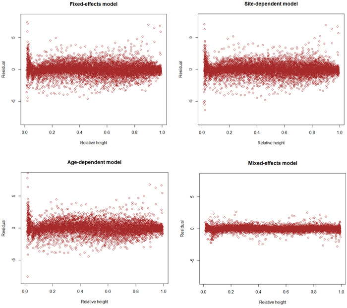
Fig. 3. Residuals of different models as a function of relative height (h/H). View larger in new window/tab.
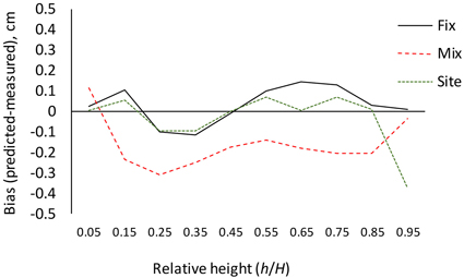
Fig. 4. Bias (predicted diameter – measured diameter) calculated for different relative heights with the fixed-effects model (Fix), fixed part of the mixed-effects model (Mix) and site index-dependent fixed-effects model (Site).
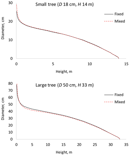
Fig. 5. Comparison of the fixed-effects model (Fixed) and fixed part of the mixed-effects model (Mixed). D is diameter at breast height; H is tree height from ground to top.
The old model (Gjølberg 1978) and our new model agree for typical combinations of dbh and height (Fig. 6, left panel) but clearly disagree for less typical shapes, for instance quickly tapering or tall and slender trees (Fig. 6, right panel).
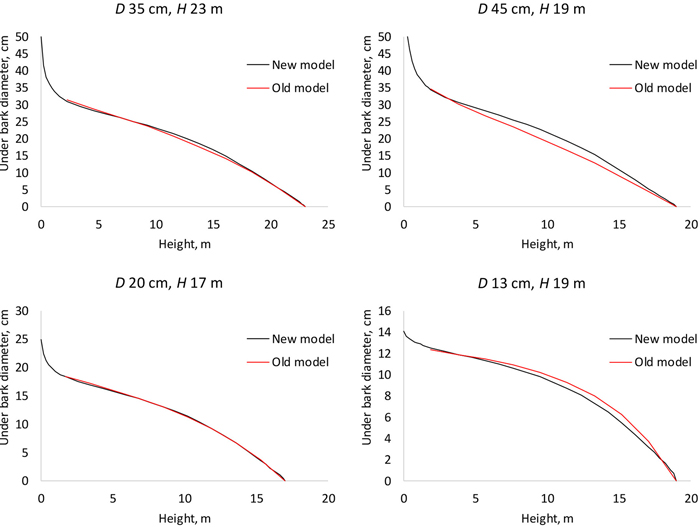
Fig. 6. Stem profiles predicted with the fixed-effects model of this study (new model) and with the model of Gjølberg 1978 (old model). D is diameter at breast height; H is tree height from ground to top.
3.6 Bark model
A model (fixed-effects Kozak 97) was fitted also for double bark thickness (Table 7). This model makes it possible to calculate stem diameter under bark, by subtracting bark thickness from over bark diameter (Fig. 7). Logically, the proportion of bark of the stem diameter was greater in small trees.
| Table 7. Parameters of the fixed-effects bark model. | ||
| Parameter | Estimate | t value |
| a0 | 0.248 | 31.9 |
| a1 | 1.060 | 55.5 |
| a2 | –0.529 | –21.1 |
| b1 | 0.379 | 15.4 |
| b2 | 0.166 | 7.3 |
| b3 | 0.275 | 2.9 |
| b4 | –0.419 | –7.9 |
| b5 | 0.025 | 9.7 |
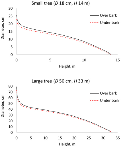
Fig. 7. Under bark diameter can be calculated by predicting bark thickness by the bark model (Table 7) and subtracting it from over bark diameter (Table 2). D is diameter at breast height; H is tree height from ground to top.
4 Discussion
This study developed a new stem taper model for Norwegian Norway spruce using a function that has been found to be among the best models for describing stem profiles (de-Miguel et al. 2012). In several studies the Kozak 02 model has been found to be best (Kozak 2004; Heiðarsson and Pukkala 2011). However, Kozak 97 and Kozak 02 are very close to each other with a consequence that their fitting statistics and predictions are also similar. Therefore, the choice between Kozak 97 and Kozak 02 is not critically important.
The model developed in this study allows predicting diameter at any height of the stem. It differs from the earlier Norwegian model (Gjølberg 1978), which consists of separate equations for different relative heights. Numerical interpolation using e.g. splines is required to calculate diameters for heights that are different from the heights for which the equations were fitted. The old model predicts only underbark diameter whereas our models can be used to predict both over- and underbark diameters. From Fig. 6 it may be concluded that our new model is valid over a wider range of diameter-height combinations, as compared to the old model.
The new model can be used, by applying simple numerical integration, to calculate the total stem volume and the volumes of various timber assortments defined by minimum log length and top diameter. The model can also be used for predicting stem diameter at any height, and for finding the height where stem diameter has a certain value.
Tree age and site index had statistically significant but small effect on stem taper. Therefore, it is possible to use those model versions in which the parameters of the baseline model depend on tree age and site index, although the improvement in the precision of volume prediction would remain small. As in the study by Arias-Rodil et al. (2015) the effect of plot (random plot factor) on stem taper was small, compared to the effects of tree-specific random parameters. The high contribution of three-specific parameters means that there is much variation between trees in stem shape. If additional diameters (besides dbh) are measured from the tree, the mixed-effects model can be calibrated for individual trees (Arias-Rodil et al. 2015). This possibility is relevant mainly in forest inventories.
One reason for the low significance of the random plot factor might be the fact that taper trees were often measured in the same plot during a long period (up to 51 years), and tree shape might have changed during this period due for instance to climate change and nitrogen deposition. One possibility to analyse potential time effects is to use measurement year as a fixed predictor of stem taper. Another possibility is to include random year effects in the model. Significant time effects would result in the need to collect new taper data continuously and update the models every now and then.
In simulation, it may not be reasonable to assume that the tree effect remains constant when the tree develops. The same tree may develop in different ways, depending on how the stand is managed in different simulations. Therefore, it may be assumed that a calibration made in the beginning of the simulation is not valid for future predictions. Thus, the mixed-effects model has limited use in simulation studies. In accordance with Arias-Rodil et al. (2015) we recommend using the fixed-effects model rather than the fixed part of the mixed-effects model when calibration data are not available.
Acknowledgements
The study was partly funded by the Norwegian Research Council trough the project “PRECISION”, project no. 281140. The authors would also like to thank former and previous colleagues at NIBIO for laborious field work through the years.
References
Arias-Rodil M., Castedo-Dorado F., Camara-Obregon A., Dieguez-Aranda U. (2015). Fitting and calibrating a multilevel mixed-effects stem taper model for maritime pine in NW Spain. PLoS ONE 10(12): 1–20. https://doi.org/10.1371/journal.pone.0143521.
Bi H.Q. (2000). Trigonometric variable-form taper equations for Australian eucalypts. Forest Science 46: 397–409.
Braastad H. (1980). Instruks og veiledning for anlegg og revisjon av forsøksfelt ved Avdeling for skogbehandling og skogproduksjon. [Instruction and guidance for establishment and revision of field trials at the Department of Forest Growth and Yield]. Norsk institutt for skogforskning, Ås. 51 p. [In Norwegian].
de-Miguel S., Mehtatalo L., Shater Z., Kraid B., Pukkala T. (2012). Evaluating marginal and conditional predictions of taper models in the absence of calibration data. Canadian Journal of Forest Research 42(7): 1383–1394. https://doi.org/10.1139/x2012-090.
Eide E., Langsæter A. (1929). Avsmalningstabell for granskog. [Table of taper for Norway spruce forests]. Meddelelser fra Det norske Skogforsøksvesen 3: 345–374. [In Norwegian with English summary].
Eide E., Langsæter A. (1954). Avsmalingstabell for granskog. Utvidet og revidert 1954. [Table of taper for Norway spruce forests. Enlarged and recomputed in 1954]. Meddelelser fra Det norske Skogforsøksvesen 12: 1–62. [In Norwegian with English summary].
Gjølberg R. (1978). Et EDB-program for analyse av verdiutviklingen for enkelttrær ved råteangrep. [A computer program for analysis of the value development of single trees attacked by root rot]. Norges landbrukshøgskole, Institutt for skogøkonomi, Notat nr. 2/78. [In Norwegian].
Heiðarsson L., Pukkala T. (2011). Taper functions for lodgepole pine (Pinus contorta) and Siberian larch (Larix sibirica) in Iceland. Icelandic Agricultural Sciences 24: 3–11.
Kozak A. (1988). A variable-exponent taper equation. Canadian Journal of Forest Research 18(11): 1363–1368. https://doi.org/10.1139/x88-213.
Kozak A. (1997). Effects of multicollinearity and autocorrelation on the variable-exponent taper functions. Canadian Journal of Forest Research 27(5): 619–629. https://doi.org/10.1139/x97-011.
Kozak A. (2004). My last words on taper equations. Forestry Chronicle 80(4): 507–515. https://doi.org/10.5558/tfc80507-4.
Kublin E., Breidenbach J., Kandler G. (2013). A flexible stem taper and volume prediction method based on mixed-effects B-spline regression. European Journal of Forest Research 132(5–6): 983–997. https://doi.org/10.1007/s10342-013-0715-0.
Muhairwe C.K., Lemay V.M., Kozak A. (1994). Effects of adding tree, stand, and site variables to Kozaks variable-exponent taper equation. Canadian Journal of Forest Research 24(2): 252–259. https://doi.org/10.1139/x94-037.
Newnham R. (1988). A variable-form taper function. Information Report PI-X-083. Petawawa National Forestry Institute, Chalk River, Ontario, Canada. 33 p.
Pinheiro J., Bates D., DebRoy S., Sarkar D., R Core Team (2018). nlme: linear and nonlinear mixed effects models. R package version 3.1-137. https://CRAN.R-project.org/package=nlme.
Pukkala T., Möykkynen T., Thor M., Rönnberg J., Stenlid J. (2005). Modeling infection and spread of Heterobasidion annosum in even-aged Fennoscandian conifer stands. Canadian Journal of Forest Research 35(1): 74–84. https://doi.org/10.1139/x04-150.
Rojo A., Perales X., Sanchez-Rodriguez F., Alvarez-Gonzalez J.G., von Gadow K. (2005). Stem taper functions for maritime pine (Pinus pinaster Ait.) in Galicia (Northwestern Spain). European Journal of Forest Research 124(3): 177–186. https://doi.org/10.1007/s10342-005-0066-6.
Sterba H. (1980). Stem curves—a review of the literature. Forestry Abstracts 41: 141–145.
Tveite B. (1977). Bonitetskurver for gran. [Site index curves for spruce]. Meddelelser fra Norsk institutt for skogforskning 33: 1–84. [In Norwegian].
Total of 19 references.
