Lauri Korhonen  ,
Jaakko Repola,
Tomi Karjalainen,
Petteri Packalen,
Matti Maltamo
,
Jaakko Repola,
Tomi Karjalainen,
Petteri Packalen,
Matti Maltamo
Transferability and calibration of airborne laser scanning based mixed-effects models to estimate the attributes of sawlog-sized Scots pines
Korhonen L., Repola J., Karjalainen T., Packalen P., Maltamo M. (2019). Transferability and calibration of airborne laser scanning based mixed-effects models to estimate the attributes of sawlog-sized Scots pines. Silva Fennica vol. 53 no. 3 article id 10179. https://doi.org/10.14214/sf.10179
Highlights
- Attributes of individual sawlog-sized pines estimated by transferring ALS-based models between sites
- Mixed effects models were more accurate than k-NN imputation tested earlier
- Calibration with a small number of field measured trees improved the accuracy.
Abstract
Airborne laser scanning (ALS) data is nowadays often available for forest inventory purposes, but adequate field data for constructing new forest attribute models for each area may be lacking. Thus there is a need to study the transferability of existing ALS-based models among different inventory areas. The objective of our study was to apply ALS-based mixed models to estimate the diameter, height and crown base height of individual sawlog sized Scots pines (Pinus sylvestris L.) at three different inventory sites in eastern Finland. Different ALS sensors and acquisition parameters were used at each site. Multivariate mixed-effects models were fitted at one site and the models were validated at two independent test sites. Validation was carried out by applying the fixed parts of the mixed models as such, and by calibrating them using 1–3 sample trees per plot. The results showed that the relative RMSEs of the predictions were 1.2–6.5 percent points larger at the test sites compared to the training site. Systematic errors of 2.4–6.2 percent points also emerged at the test sites. However, both the RMSEs and the systematic errors decreased with calibration. The results showed that mixed-effects models of individual tree attributes can be successfully transferred and calibrated to other ALS inventory areas in a level of accuracy that appears suitable for practical applications.
Keywords
Pinus sylvestris;
LIDAR;
crown base height;
hierarchical data;
individual tree detection;
sawlog quality
-
Korhonen,
University of Eastern Finland, School of Forest Sciences, P.O. Box 111, FI-80101 Joensuu, Finland
 http://orcid.org/0000-0002-9352-0114
E-mail
lauri.korhonen@uef.fi
http://orcid.org/0000-0002-9352-0114
E-mail
lauri.korhonen@uef.fi
- Repola, Natural Resources Institute of Finland (Luke), Natural resources, Eteläranta 55, FI-96300 Rovaniemi, Finland E-mail jaakko.repola@luke.fi
- Karjalainen, University of Eastern Finland, School of Forest Sciences, P.O. Box 111, FI-80101 Joensuu, Finland E-mail tomikar@uef.fi
- Packalen, University of Eastern Finland, School of Forest Sciences, P.O. Box 111, FI-80101 Joensuu, Finland E-mail petteri.packalen@uef.fi
- Maltamo, University of Eastern Finland, School of Forest Sciences, P.O. Box 111, FI-80101 Joensuu, Finland E-mail matti.maltamo@uef.fi
Received 17 April 2019 Accepted 31 July 2019 Published 5 August 2019
Views 88771
Available at https://doi.org/10.14214/sf.10179 | Download PDF

1 Introduction
Sawlogs are generally the most valuable forest product, and their quality attributes are of great interest in practical wood procurement. In the 1980s pre-harvest inventories of marked stands were routinely performed in Finland to obtain more information about sawlog quality, but later the costs of such inventories became too large for the system to be profitable. The use of airborne laser scanning (ALS) data in forest inventories, however, facilitates the prediction of pre-harvest information without having to measure every tree in the field (Peuhkurinen et al. 2007; Korhonen et al. 2008).
ALS-based forest inventories rely on models where tree and stand attributes are estimated using ALS metrics as predictor variables. The role of the models is to predict the attributes of interest over the whole inventory area. These models are constructed using local GNSS-positioned field data acquired from the inventory area. In the area based approach (ABA), the models are based on the statistical relationship between ALS metrics and stand attributes at the plot level. Individual tree detection (ITD) applications require ALS-based models for the estimation of the detected trees’ attributes, such as diameter, volume and biomass. Individual tree detection is most promising for mature stands that have been managed with thinnings, because almost all trees can be detected reliably due to the small variation in heights and the regular spatial pattern of trees. Thus, ITD is potentially well suited for acquiring information about sawlog properties (Vastaranta et al. 2014). In addition to tree species and the diameter at breast height (DBH), the height of the living base of the crown (CBH) is directly related to the value of sawlogs. Studies from Finland indicated that it is possible to estimate CBH from ALS data with an accuracy of 1–1.5 m (Vauhkonen 2010; Maltamo et al. 2018), but thus far the CBH has not been estimated in practical inventories.
The models applied in practical inventories are generally constructed using regression analysis or non-parametric methods, such as k nearest neighbor (k-nn). However, the development of suitable prediction methods remains as a primary issue in forest inventory research. One common case where more advanced statistical models are needed is a situation where the data exhibits internal correlations or hierarchies. For example, spatial correlations exist when tree properties are more strongly correlated within stands than among stands, and measuring multiple trees from each stand thus results in hierarchical data. Such correlation structures need to be addressed correctly in order to obtain a flexible model structure and reliable standard error estimates for the parameters (Parresol 1999; Parresol 2001). Hierarchically structured data can be analyzed by using mixed effects models, which permit an analysis of between stand and within stand variations. Mixed-effects models can also be calibrated to a new stand with just a few new measurements, and the information about between and within stand variations can be utilized in the process (McCulloch and Searle 2001). In an ALS inventory context, mixed-effects models have been applied both at ABA (Breidenbach et al. 2008) and ITD studies (Salas et al. 2010; Maltamo et al. 2012).
Multivariate mixed-effects models comprise a set of linear sub-models, and can be applied to estimate several responses simultaneously. This procedure enables the transfer of information from one sub-model to another, and across-model correlations can be utilized while calibrating models to new stands (Lappi 1991). In multivariate mixed-effects models, a calibration of one sub-model can also affect the predictions of other sub-models. In ALS inventory cases, such flexible calibration is an attractive possibility, since ALS data are available wall-to-wall and additional calibration measurements can be made at stands of specific interest. For example, Maltamo et al. (2012) calibrated an ALS-based multivariate tree attribute model to a new stand within the same inventory area using additional measurements of DBH, CBH, and tree height (H). In addition, tree volume was calibrated by utilizing the random cross-variate covariate structure of the model.
The transferability of the constructed models is another important feature. Typically, in practical ALS-based forest inventories, field and ALS data are acquired simultaneously and new models are constructed for each site from which ALS data are collected. However, nowadays it is common in many countries that dense ALS data have been collected for other purposes, but field measurements required for forest inventory are lacking. In such cases an old model that was constructed with another ALS data set could be applied (Uuttera et al. 2006; Tompalski et al. 2019). However, the model may not perform as well in a new site, because the ALS sensor and scanning parameters may differ among the inventory areas, which could cause systematic differences in ALS metrics estimated from the data (Hopkinson 2007; Næsset 2009). Furthermore, datasets may also be collected under leaf-off or leaf-on conditions, and there could also be variations in stand structures or types of vegetation (Næsset 2002; Næsset 2005; Kotivuori et al. 2016). Thus, model transfers are usually avoided if the objective is to conduct an unbiased inventory of forest resources. Sometimes the information obtained from an earlier model may nevertheless be useful in decision making, because several studies have shown that the decreases in accuracy are often moderate (Uuttera et al. 2006; Karjalainen et al. 2019; Tompalski et al. 2019). Another approach is to combine several ALS inventory areas to construct general large-area models for the prediction of stand attributes (Næsset and Gobakken 2008; Nilsson et al. 2017; Kotivuori et al. 2018; Noordermeer et al. 2019). Such models already incorporate data from multiple inventories and ALS sensors, which could result in more reliable estimates as the model coefficients are less dependent on individual sites and sensors.
The objective of our study was to estimate DBH, H and CBH of sawlog-sized Scots pines (Pinus sylvestris L.) at two separate test areas by applying ALS-based models constructed at an external training area. The steps required to reach the objective were: (i) to model the tree-level attributes using a multivariate mixed-effects model in a training area, (ii) to validate the fixed parts of the sub-models in two separate test areas in which the ALS data have been collected with different sensors and parameter settings than in the training data, (iii) to calibrate the constructed models in the separate test areas using a small number of field measured trees, and (iv) to compare the accuracies of the estimated attributes to those reported in earlier studies.
2 Materials
2.1 Field data
We used a data set consisting of sawlog sized Scots pines from Liperi, Eastern Finland, to construct multivariate mixed-effect models for DBH, H and CBH. Two other data sets consisting of sawlog sized Scots pines, Kiihtelysvaara and Koli, were used as test areas for validating the transferability of the models. Both test areas were located ≤100 km from the Liperi area (Fig. 1). Each plot consisted of sawlog-sized, more or less even-aged trees, and Scots pine was the dominant species. In Liperi and Kiihtelysvaara, the forests were privately owned. In contrast, the Koli plots were located inside the Koli National Park where silvicultural operations had not occurred since 1991. The silvicultural inactivity may have caused differences in vegetation structure between Koli and the other two areas.
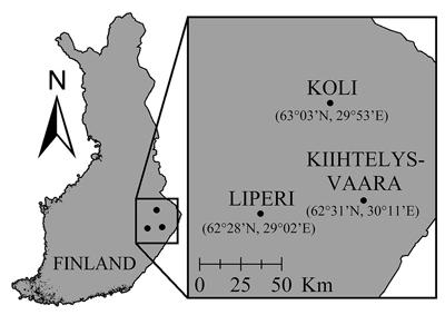
Fig. 1. Locations of the Liperi training site and the Kiihtelysvaara and Koli test sites. In Liperi, the field plots were located max. 20 km away from the presented point, whereas in Kiihtelysvaara and Koli sites, all plots were located <3 km away from the presented points.
The Liperi field data were collected in summer 2017. There were a total of 47 plots and the plot size was 30 × 30 m. DBH, CBH and H of every tree with DBH > 5 cm were measured regardless of the species. The CBH was defined as the height of the base of the lowest living branch in the living crown. The locations of the trees were determined using the method presented by Korpela et al. (2007). The Kiihtelysvaara test site had 66 plots that were measured in 2010 and the measurements were similar to Liperi, except that the plot sizes were 20 × 20 m, 25 × 25 m, or 30 × 30 m depending on tree height and density. In the Koli test site, 14 plots of size 30 × 30 m were measured in 2006 and the measurement procedure was similar to Liperi and Kiihtelysvaara, with the exception that the tree positions were determined in the field based on GPS-positioned plot corners. However, only Scots pines with DBH ≥ 16 cm that were detected unambiguously from ALS data (see below) were included into the data sets, while all other trees were omitted. We did not consider the tree detection rate or species classification, as our focus was on predicting the attributes of sawlog-sized Scots pines that could be detected reliably, which is a realistic scenario in pre-harvest inventory of marked stands. The Liperi data consisted of 1051 Scots pines, while the test datasets in Kiihtelysvaara and Koli had of 414 and 317 Scots pines, selected as in Liperi (Table 1).
| Table 1. Attributes of Scots pines used for training (Liperi site) and testing (Kiihtelysvaara and Koli sites) the mixed effect models. N = number, DBH = diameter at breast height, H = height, CBH = Crown base height. The range of values is given in parentheses. | ||||||
| Site | Coordinates | Nplot | Ntree | Mean DBH, cm | Mean H, m | Mean CBH, m |
| Liperi | 62°28´N, 29°02´E | 47 | 1051 | 24.8 (17.0–48.1) | 21.2 (12.4–35.6) | 13.3 (5.1–27.3) |
| Kiihtelysvaara | 62°31´N, 30°11´E | 66 | 414 | 23.1 (16.0–42.8) | 19.5 (12.3–34.3) | 11.0 (3.7–24.3) |
| Koli | 63°03´N, 29°53´E | 14 | 317 | 24.6 (16.1–44.4) | 19.9 (11.2–28.8) | 11.2 (2.8–21.8) |
2.2 ALS data and its processing
Each inventory area was scanned in leaf-on conditions, but with different sensors and scanning parameters (Table 2). The Optech Titan scanner that was used in Liperi provided multispectral ALS data at three wavelengths, but we only used the 1064 nm channel in this study.
| Table 2. Details of the laser scanning data obtained from the training (Liperi) and test (Kiihtelysvaara and Koli) sites. | |||
| Site | Liperi | Kiihtelysvaara | Koli |
| Scanning time (month/year) | 7/2016 | 6/2009 | 7/2005 |
| Sensor type | Optech Titan | Optech ALTM Gemini | Optech ALTM 3100 |
| Flying altitude (m) | 850 | 600 | 900 |
| Scanning angle (°) | 40 | 26 | 22 |
| Pulse frequency (kHz) | 250 | 100 | 100 |
| Overlap (%) | 55 | 55 | 35 |
| Strip width on ground (m) | 650 | 320 | 350 |
| Mean pulse density (m–2) | 13.2 | 14.7 | 5.2 |
| Echoes/crown (First) | 243 | 276 | 147 |
| Echoes/crown (Last) | 74 | 90 | 75 |
Canopy height models (CHMs) that describe the height of the canopy layer above ground level were first constructed from the ALS data (Hyyppä et al. 2001). We applied the method presented by Isenburg (2014) and Khosravipour et al. (2014) to obtain CHMs at a resolution of 0.333 m. The method is based on the construction of multiple CHMs that use ALS echoes from different height ranges, and in the end the CHMs are stacked to obtain a single CHM that is free of empty pixels (Isenburg 2014). The trees were detected from the CHM with the rLiDAR-package (Silva et al. 2017) available for the statistical computing environment R (R Core Team 2016). The CHM was first low-pass filtered (Gaussian-filter; sigma value 0.6) to reduce the number of small peaks in the CHM, which subsequently decreased the number of false trees detected from the CHM. We assumed that the local maxima of the CHM represented tree tops, and detected these peaks using the rLiDAR function FindTreesCHM. The crowns were then segmented based on the local maxima using the rLiDAR function ForestCAS, which implements tree boundary delineation from the CHM. Because we were only interested in sawlog-sized Scots pines, crown segmentation was limited by setting the minimum height of the local maxima at 8 m and the maximum crown radius at 4 m. In addition, we only allowed pixels with a height value > 0.5 × the detected height of the tree to be included in the segments. The segmentation was executed with the same parameters on each plot.
The field-measured trees were linked to the respective segments. Small understory trees were ignored in the process. If a tree segment contained multiple non-understory trees, the whole segment was omitted, because we wanted the segmented ALS echoes to only link with one large and unambiguously detected tree (Maltamo et al. 2012; Karjalainen et al. 2019). The presence of multiple large trees within a segment would have distorted the relationships between the ALS metrics and tree attributes. Segments containing species other than Scots pine were omitted. In Liperi, Kiihtelysvaara and Koli, the fractions of segments with sawlog-sized trees that were omitted from the analyses due to these reasons were 10%, 8% and 35%, respectively. The percentage was especially large for the Koli site due to the lack of silvicultural operations in the national park.
The echoes located inside the final segments were used to compute a set of tree level ALS metrics separately for first (first of many + only) and last (last of many + only) echoes. In addition, a set of similar plot-level metrics was computed using first echoes. Thus, the values of the plot-level metrics were the same for each tree within the plot. Plot-level ALS metrics contained information with regard to the surroundings of the individual trees, such as tree density and mean height, which could also influence the crown shapes of the trees. The metrics were based on height and intensity distributions of the echoes, including maximums, minimums, means, medians, modes, variances, standard deviations, coefficients of variation, skewness and kurtosis values (Table 3). Of the intensity metrics, only kurtosis, skewness and the coefficient of variation were observed to be similar between the inventory areas, and therefore the other intensity metrics were excluded from further analyses.
| Table 3. A list of the predictor variables extracted from airborne laser scanning data. In the height percentiles, i = 5, 10, 15…80, 90, 95 and 99. | ||
| ALS metric | Definition | Computed for |
| TotalReturns | Total number of returns | Trees |
| TotalFirst | Total number of first returns | Plots |
| EWIDTH/NWIDTH | Tree crown width and depth | Trees |
| HMAX | Maximum height | Trees & plots |
| HMIN | Minimum height | Plots |
| HMEDIAN | Median height | Trees & plots |
| HMEAN | Mean height | Trees & plots |
| HSD | Standard deviation of heights | Trees & plots |
| HCV | Coefficient of variation of heights | Trees & plots |
| ICV | Coefficient of variation of intensities | Trees & plots |
| HMOD | Mode of heights | Trees & plots |
| H01TH | 1st percentile of heights | Plots |
| HiTH | ith percentile of heights | Trees & plots |
| HVAR | Variance of heights | Trees & plots |
| HKUR | Kurtosis of heights | Trees & plots |
| IKUR | Kurtosis of intensities | Trees & plots |
| HSKE | Skewness of heights | Trees & plots |
| ISKE | Skewness of intensities | Trees & plots |
| CRR | Canopy relief ratio | Plots |
3 Methods
3.1 Mixed effects modeling
The DBH, H, and CBH were modelled using tree and plot level ALS metrics as predictor variables. In practical applications stand is the basic unit of model calibration, but in this study we assumed that a plot represents an entire stand. The basic assumption in our modeling approach was that the tree variables, i.e. DBH, H, and CBH, are correlated within same plot and the same tree. This entails both spatial (hierarchical data structure) and contemporaneous correlation, i.e. statistical dependency among the sub-models so that individual model errors are correlated both at plot and tree levels. Multivariate procedures with random plot and tree effects were applied to take into account both spatial and across-model (contemporaneous) correlations. First, the models were fitted independently for each response variable in order to find the significant predictors. Then a set of linear sub-models was constructed to form a multivariate linear mixed effects model, where the parameters of all sub-models were estimated simultaneously. Linear models were selected based on the linear relationship between tree attributes and ALS metrics, and the knowledge of previous studies conducted in the similar boreal growing conditions (Næsset and Økland 2002; Vauhkonen 2010; Maltamo et al. 2012).
Variable selection was based on 5% significance level and the –2×loglikelihood value of the model. The data were hierarchically (2-level) structured and the multivariate model was constructed as follows:
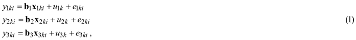
where:
y1ki, y2ki, y3ki = response tree variables DBH, H and CBH for tree i in plot k
1, 2, 3 = indices of the response variables
x1ki, x2ki, x3ki = vectors of the predictor variables for tree i in plot k
b1, b2, b3 = vectors of the fixed effects parameters
u1k, u2k, u3k = random effect for plot k
e1ki, e2ki, e3ki = residual error for tree i in plot k
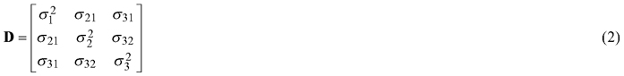
The covariances of random parameter estimates (cov(unk,un+1k)) and residual errors (cov(enki,en+1ki)) were estimated. All the random parameters (u1k, u2k, u3k) of the same plot were correlated with each other, and the residual errors (e1ki, e2ki, e3ki) of the same tree were also correlated. The random parameters and residuals were assumed to be uncorrelated Gaussian random variables with a mean of zero. In addition, the covariance structure of the random parameters (u1k, u2k, u3k) was assumed to be unstructured by enabling different variances and covariances. Thus, the covariance matrix of random effects (D) can be described in general form as:
The MIXED procedures of SAS (SAS Institute 1999) were used to estimate the multivariate model with several responses.
3.2 Model validation
In the model validation, the predicted DHB, H and CBH were evaluated against the test data (Kiihtelysvaara and Koli sites) by applying the compiled sub-models (Eq. 1). In the prediction phase, either the fixed effects or the fixed and random plot effects were used. In the fixed predictions (ŷfixed) only predictor variables of the new ALS data were used (Eq. 3), whereas in the calibrated predictions (ŷcalib) random plot effects were also considered (Eq. 4):
![]()
![]()
where ![]() is the vector of estimated fixed effects parameters, xki is the vector of predictor variables, and
is the vector of estimated fixed effects parameters, xki is the vector of predictor variables, and ![]() are the predicted random plot effects. The calibration was carried out with field measurements of 1, 2 or 3 sample trees per plot. The sample tree selection was based on tree diameter; trees with a minimum (DBHmin), maximum (DBHmax), and median (DBHmed) diameter from each plot were tested as calibration trees. These are realistic options for the calibration – if it is possible to visit the stand of interest to gather data for calibration, it will be easy to define the trees with approximate minimum, median and maximum diameters visually.
are the predicted random plot effects. The calibration was carried out with field measurements of 1, 2 or 3 sample trees per plot. The sample tree selection was based on tree diameter; trees with a minimum (DBHmin), maximum (DBHmax), and median (DBHmed) diameter from each plot were tested as calibration trees. These are realistic options for the calibration – if it is possible to visit the stand of interest to gather data for calibration, it will be easy to define the trees with approximate minimum, median and maximum diameters visually.
Random plot effects for each response variable of the multivariate model (Eq. 1) were predicted (Eq. 5) as follows (Lappi 1991; McCulloch and Searle 2001):
![]()
where ![]() is p×1 vector of the random plot effects, Z is n×p design matrix of random variables containing only dummy variable 0/1 by plots, R is n×n diagonal matrix of residual errors, D is p×p covariance matrix of random parameters with diagonal structure, yobs is n×1 vector of observed values of the dependent variable (DBH, H or CBH), and ŷfixed is n×1 vector of predicted fixed effects for DBH, H or CBH. In the above notations, p is the number of random plot effects, and n is the number of sample trees.
is p×1 vector of the random plot effects, Z is n×p design matrix of random variables containing only dummy variable 0/1 by plots, R is n×n diagonal matrix of residual errors, D is p×p covariance matrix of random parameters with diagonal structure, yobs is n×1 vector of observed values of the dependent variable (DBH, H or CBH), and ŷfixed is n×1 vector of predicted fixed effects for DBH, H or CBH. In the above notations, p is the number of random plot effects, and n is the number of sample trees.
The model validation was based on the root mean squared error (RMSE) value and the mean difference (MD) (Eq. 6 and 7) as follows:


where y is the observed value, ŷ is the predicted value (ŷfixed or ŷcalib) and N is the number of observations. To facilitate comparisons with earlier studies, we also computed relative RMSE (RMSE-%) and MD (MD-%) for each variable by dividing the RMSE or MD by the mean of the attribute within the data set.
4 Results
4.1 Multivariate model
The multivariate linear mixed-effects model contained the sub-models for DBH, H and CBH. In addition to fixed effects, all sub-models contained random effects that also included across-model covariance both at plot and tree levels (Table 4). Fixed effects were based only on tree and plot level ALS metrics. The sub-model for H was based on two tree-level ALS metrics, whereas the sub-models for DBH and CBH contained a larger number of ALS metrics including plot-level metrics. Each sub-model contained 1–2 tree level height metrics, and the sub-model for CBH also included the mean height of all echoes within the plot. Crown width (EWIDTH) and depth (NWIDTH) were significant predictors of the main effect for DBH, and EWIDTH was significant as an interaction term with tree level HMEAN for CBH. Both tree level skewness (ISKE) and kurtosis (IKUR) of intensity distribution were included in the DBH model. The RMSE values obtained for DBH, H and CBH were 2.7 cm, 0.6 m, and 1.6 m, respectively.
| Table 4. Parameter estimates of the mixed effects models for diameter at breast height (DBH), height (H), and crown base height (CBH). For the fixed parameters, the standard error is given in parentheses. Subscripts t and p denote tree and plot level metrics, respectively. Variances and covariances of random parameters (unk) and residual errors (enki) are given (correlation shown in parenthesis). The abbreviations of the predictors are explained in Table 3. | |||
| Predictor | DBH, cm | H, m | CBH, m |
| Intercept | 28.284 (10.071) | 1.756 (0.178) | –0.466 (0.593) |
| H50t | 0.660 (0.032) | ||
| H90t | 0.523 (0.041) | ||
| H95t | 2.154 (0.265) | ||
| ln(H95t) | –18.664 (5.057) | ||
| HMAXt | 0.460 (0.039) | ||
| HMEANp | 0.237 (0.062) | ||
| ln(NWIDTH) | 2.313 (0.330) | ||
| EWIDTH | 2.121 (0.378) | ||
| EWIDTH2 | –0.128 (0.035) | ||
| H70p | –0.009 (0.002) | ||
| ISKEt | –4.425 (0.420) | 1.309 (0.207) | |
| IKURt | 1.113 (0.206) | –0.367 (0.101) | |
| HMEANt/EWIDTH | 0.151 (0.047) | ||
| Random effects | |||
| var(unk) | 0.818 | 0.071 | 0.976 |
| cov(unk,un+1k) | u1k | u2k | u3k |
| u2k | 0.066 (0.273) | ||
| u3k | –0.159 (–0.178) | 0.083 (0.315) | |
| var(enki) | 6.644 | 0.310 | 1.556 |
| cov(enki,en+1ki) | e1ki | e2ki | e3ki |
| e2ki | 0.069 (0.048) | ||
| e3ki | –0.809 (–0.252) | 0.048 (0.069) | |
Statistical dependence or across-model correlation among the sub-models was detected at both plot and tree levels. The correlations were small but larger at the plot level than at the tree level. The CBH showed the greatest across-model correlation at the plot level with H (0.315) and DBH (0.273) (Table 4).
4.2 Model validation with fixed predictions
The sub-models (Eq. 1) were applied to evaluate DBH, H and CBH predictions against the observations from the Kiihtelysvaara and Koli test areas (Table 5). The RMSE values increased by 1.2–2.8 (Kiihtelysvaara) or 3.6–6.5 (Koli) percent points, i.e. the estimation was more reliable at the Kiihtelysvaara site. In general, the fixed predictions were considerably more reliable for H (RMSE 5.6–6.4%) than DBH (RMSE 13.4–15.9%) or CBH (RMSE 13.3–18.5%) (Figs. 2–4). In Kiihtelysvaara, the DBH predictions were, on average, overestimated (MD: –1.3 cm or –5.7%), and H and CBH predictions were, on average, underestimated (MD: 0.61 m or 3.1%, and 0.68 m or 6.2%, respectively) (Table 5). In Koli, the predictions were, on average, overestimated, and the MDs were –1.3 cm (–5.4%), –0.48 m (–2.4%) and –0.65 m (–5.8%) for DBH, H and CBH, respectively.
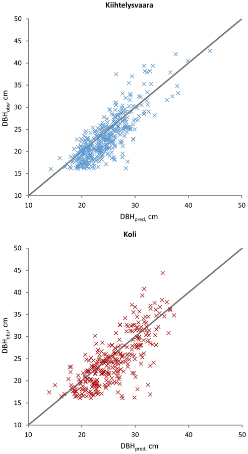
Fig. 2. Observed (DBHobs) versus predicted (DBHpred) Scots pine diameters in the Kiihtelysvaara and Koli test sites. The predicted values were obtained with the fixed part of the mixed model trained at the Liperi site.
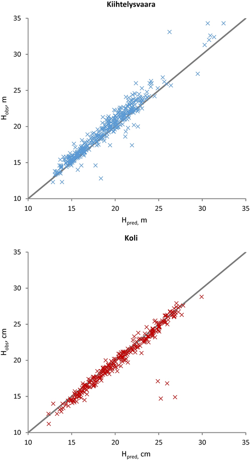
Fig. 3. Observed (Hobs) versus predicted (Hpred) Scots pine heights at the Kiihtelysvaara and Koli test sites. The predicted values were obtained with the fixed part of the mixed model trained at the Liperi site.
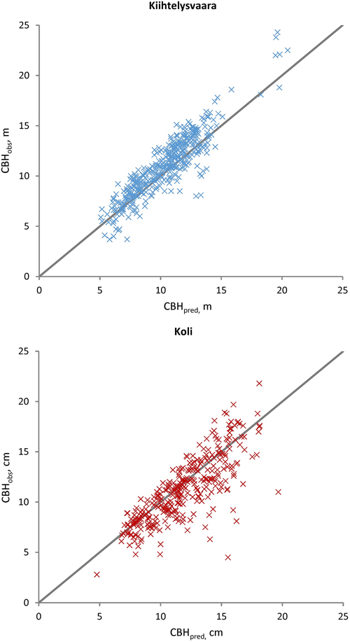
Fig. 4. Observed (CBHobs) versus predicted (CBHpred) Scots pine crown base heights at the Kiihtelysvaara and Koli test sites. The predicted values were obtained with the fixed part of the mixed model trained at the Liperi site.
| Table 5. Root mean square errors (RMSE) and mean differences (MD) between the observed diameter at breast height (DBH), height (H), and crown base height (CBH) and the estimates obtained from the mixed effects models. The results are shown for the training site (Liperi) and for the two test sites (Kiihtelysvaara and Koli). Calibrations were made at the test sites using the pines with minimum and median diameters. | ||||
| Liperi | Kiihtelysvaara | Koli | ||
| DBH | RMSE, cm | 2.7 | 3.1 | 3.91 |
| RMSE% | 10.9 | 13.4 | 15.9 | |
| RMSE calibrated, cm | 2.87 | 3.58 | ||
| RMSE% calibrated | 12.4 | 14.6 | ||
| MD, cm | 0 | –1.3 | –1.3 | |
| MD% | 0 | –5.7 | –5.4 | |
| MD calibrated, cm | –0.77 | –0.7 | ||
| MD% calibrated | –3.3 | –2.8 | ||
| H | RMSE, m | 0.6 | 1.09 | 1.28 |
| RMSE%, m | 2.8 | 5.6 | 6.4 | |
| RMSE calibrated, m | 0.99 | 1.16 | ||
| RMSE% calibrated | 5.1 | 5.8 | ||
| MD, m | 0 | 0.61 | –0.48 | |
| MD% | 0 | 3.1 | –2.4 | |
| MD calibrated, m | 0.51 | –0.22 | ||
| MD% calibrated | 2.6 | –1.1 | ||
| CBH | RMSE, m | 1.6 | 1.46 | 2.07 |
| RMSE% | 12.0 | 13.3 | 18.5 | |
| RMSE calibrated, m | 1.26 | 1.9 | ||
| RMSE% calibrated | 11.5 | 17.0 | ||
| MD fixed, m | 0 | 0.68 | –0.65 | |
| MD% fixed | 0 | 6.2 | –5.8 | |
| MD calibrated, m | 0.24 | –0.33 | ||
| MD% calibrated | 2.2 | –2.9 | ||
4.3 Model validation with calibrated predictions
The calibrated predictions (ŷcalib) were obtained by predicting random plot effects with 1–3 field measured sample trees. Calibration using the measured median or minimum diameter of the pines improved the predictions for all response variables: the relative RMSEs decreased on average by 0.9 percent points, depending on the variable, compared to the predictions made with the fixed part. Calibration was overall most efficient with the minimum diameter, while using the maximum diameter sometimes even increased the RMSE compared with the mixed part. However, even smaller RMSEs were obtained with two or three calibration trees. Overall the best combination was to use the trees with minimum and median diameters from each plot. This calibration decreased the RMSEs on average by 1.1 percent points compared to the fixed part (Table 5). Calibration with three sample trees (minimum, median, and maximum diameter) did not provide further improvements.
In terms of absolute decrease in RMSE-%, the calibration effect was largest for CBH (RMSE from 13.3–18.5% to 11.5–17.0%), average for DBH (RMSE from 13.4–15.9% to 12.4–14.6%) and smallest for H (RMSE from 5.6–6.4% to 5.1–5.8%). However, the calibrations especially affected MD. The MD of CBH decreased from 0.68 m to 0.24 m in Kiihtelysvaara, and from –0.65 m to –0.33 m in Koli (Table 5). Correspondently, the MD values of H decreased from –0.61 m to –0.51 m in Kiihtelysvaara, and from –0.48 m to 0.22 m in Koli. The calibration effect was smallest for the MD of DBH, as the values decreased from –1.3 to –0.77 cm and from –1.3 to –0.7 cm in Kiihtelysvaara and Koli, respectively.
5 Discussion
This study examined multivariate mixed-effects modelling and calibration of DBH, H and CBH of sawlog-sized Scots pines. Those attributes were initially modelled using ALS-based predictive variables, and the constructed multivariate models were calibrated for other ALS inventory areas using field measurements of DBH, H and CBH obtained from 1–3 trees. We only considered sawlog-sized Scots pines, since they usually form the most valuable part of the tree stock, and such trees can usually be detected ALS data without frequent omission or commission errors. We did not consider detection rates or tree species recognition, as our main focus in this study was on the transferability and calibration of the models. However, we acknowledge that in practical applications tree detection may be the limiting factor, especially if the stand has not been managed with thinnings. This must be taken into consideration when interpreting results of this study.
The modelling of tree attributes was based on ALS metrics from the Liperi training area. The accuracies obtained for DBH, H and CBH in Liperi were 2.7 cm, 0.6 m and 1.6 m, respectively. These values are slightly smaller than the values obtained by Karjalainen et al. (2019) using the k-nn approach with the same data sets (i.e. 3.4 cm, 0.9 m and 1.8 m). It was expected that mixed-effects modelling leads to improved accuracy, since the k-nn results were based on the simultaneous estimation of five tree variables (volume and sawlog volume were also included), whereas the predictors in our multivariate model were selected separately for each response variable. Our DBH sub-model included a total of eight ALS predictors, which is a relatively large number. In comparison, Karjalainen et al. (2019) included 5–7 predictors in their k-nn models.
The RMSE values for tree attribute predictions using the fixed parts of the sub-models showed an increase in the test areas with respect to the training data, especially in Koli, but the changes were not substantial. In general, the RMSE values obtained by Karjalainen et al. (2019) using k-nn were slightly larger for DBH in both areas, and for CBH in Koli. However, when MD values are compared, the results are contradictory (over- or underestimates), especially in the case of H. However, the magnitude of systematic differences was rather small. It would thus seem that multivariate mixed-effects models can be transferred with smaller errors than k-nn models. It is obvious that dramatic changes in accuracy are not expected if the mixed-effects models are transferred between ALS inventory areas, provided that the growing conditions of the forests remain more or less the same (see also Breidenbach et al. 2008).
Compared with using just the fixed parts, calibrations conducted with the tree variables measured in the field showed slight decreases in RMSE in most cases and behaved logically in relation to the amount of calibration information, both with regard to RMSE and MD. For example, the measurements of DBH, H and CBH in Kiihtelysvaara decreased the RMSE values by 0.2 cm, 0.1 m and 0.2 m, respectively. Thus, the effect of calibration was comparable to the study by Maltamo et al. (2012), where a similar type of calibration was conducted within a single ALS inventory area. This further shows the robustness of the mixed-modelling approach in conditions where the properties of the predictor variables change.
In this study, the models for DBH, H and CBH were estimated by applying a multivariate mixed-effects model rather than estimating each model independently. This procedure enables a more flexible model calibration to a new stand, particularly if statistical dependence exists among the sub-models (across-model correlations). A prerequisite for effective model calibration is that the random parameters among the sub-models are correlated. Under these circumstances, information can be transferred effectively from one model to another, and the calibration can be applied by utilizing the across-model correlations and measurements of other response variables (Lappi 1991). This would enable model calibration, for example, using only DBH measurements (the primary tree variable used in forest inventories). We examined this approach by selecting only DBH for the calibration of H and CBH sub-models. The effect of the across-model calibration was relatively minor, and the improvement in accuracy (RMSE, MD) of the H and CBH predictions, compared to fixed predictions, was very small (data not shown), because the random plot parameters among the sub-models exhibited weak correlations. Therefore, it was more effective to use field measured response variables (DBH, H and CBH) for the calibration, rather than only using DBH.
The RMSEs that we observed after calibration (DBH 12.4–14.6%, H 5.1–5.8%, CBH 11.5–17.0%) are clearly larger than the ones obtained locally at the Koli site (Maltamo et al. 2009) using k-nn models (5.2%, 2.0%, and 7.1% for DBH, H and CBH of Scots pines, respectively). However, Vauhkonen et al. (2014) reported RMSEs of 14%, 4% and 13%, respectively, at the Kiihtelysvaara site for unambiguously detected trees. Those values are similar to our calibrated RMSEs, but it should be noted though that their data included also other species and size classes. Our estimates also contained systematic errors (MD%: DBH 5.4–5.7%, H 2.4–3.1%, CBH 6.2–5.8%), although we did not observe any lack-of-fit in the training data based on the inspection of residual plots. Thus, the systematic errors in the test data were probably caused by variations in ALS data and vegetation structure among the areas.
Although errors in forest inventory data are always detrimental from an operational perspective, the observed error levels are not especially large compared to other forest management inventories. For example, systematic prediction errors observed in species specific ABA inventories can be about 10% for mean DBH and H, when the estimation is performed for external validation data (Maltamo et al. 2009; Wallenius et al. 2012). The RMSEs obtained for stand volume in relascope-based management inventories applied in large areas before the introduction of ALS were commonly > 20% (Haara and Korhonen 2004). These values are clearly larger than the MDs and RMSEs and reported here. The errors obtained for individual trees in the field-based studies are considerably smaller than those reported here, e.g. Päivinen et al. (1992) reported an error of 0.7 cm for DBH, but it is obvious that remotely sensed estimates cannot reach similar accuracies as field measurements.
Despite the observed inaccuracies, we consider our results promising for practical applications. From a practical perspective, the results should be assessed using methods that consider the value of information (Kangas et al. 2014). If ALS data are available, it is possible to apply our models with very small costs, because the fixed parts of the sub-models can be applied without additional field work. The cost of measuring a few sample trees for calibration is also minor compared to constructing local ITD models, where tree coordinates are needed together with the actual attributes of interest. The CBH for example is currently lacking from the practical inventory products in Finland, although it is one the most important sawlog quality attributes. Further research is needed to determine the value of remotely sensed tree level information from the perspective of commercial forestry.
6 Conclusions
This study showed that tree attribute models of sawlog-sized Scots pine trees constructed with a multivariate mixed-effects modeling approach, by applying ALS metrics as predictor variables, can be transferred to other ALS inventory areas scanned with different ALS sensor and parameter settings with only moderate increases in RMSE (1.2–6.5 percent points). Constructed models can be localized to a new stand in a new area by measuring a small number of calibration trees, which decreases the systematic errors caused by the model transfer. The calibration approach offers a cost-effective method for obtaining tree-level pre-harvest information of timber quality attributes such as DBH (RMSE = 2.9–3.6 cm) and CBH (RMSE = 1.0–1.2 m) in areas where ALS data are available but sufficient field measurements for constructing new models are lacking. The DBH of the smallest sawlog-sized Scots pine measured from the plot was the most efficient calibration variable, but also the DBH of the median tree could be measured for smaller RMSE. The models could also be applied in new areas without calibration, albeit with larger errors (DBH RMSE = 3.1–3.9 cm, CBH RMSE = 1.5–2.1 m). The results indicate that mixed-effects models are robust in conditions where the properties of the ALS-based predictor variables change due to different sensor configurations. However, the method assumes that all trees are detected without errors, which may be an issue in multilayered stands.
Acknowledgements
The study was funded by the Ministry of Agriculture of Finland through the project “Measurement and modelling of tree quality”. We wish to thank the anonymous reviewers for their helpful comments.
References
Breidenbach J., Kublin E., McGaughey R.J., Andersen H.E., Reutebuch S.E. (2008). Mixed-effects models for estimating stand volume by means of small footprint airborne laser scanner data. Photogrammetric Journal of Finland 21: 4–15.
Haara A., Korhonen K.T. (2004). Kuvioittaisen arvioinnin luotettavuus. Metsätieteen aikakauskirja 4: 489–508. https://doi.org/10.14214/ma.5667.
Hopkinson C. (2007). The influence of flying altitude, beam divergence, and pulse repetition frequency on laser pulse return intensity and canopy frequency distribution. Canadian Journal of Remote Sensing 33(4): 311–324. https://doi.org/10.5589/m07-029.
Hyyppä J., Kelle O., Lehikoinen M., Inkinen M. (2001). A segmentation-based method to retrieve stem volume estimates from 3-D tree height models produced by laser scanners. IEEE Transactions on Geoscience and Remote Sensing 39(5): 969–975. https://doi.org/10.1109/36.921414.
Isenburg M. (2014). Rasterizing perfect Canopy Height Models from LiDAR. https://rapidlasso.com/2014/11/04/rasterizing-perfect-canopy-height-models-from-lidar/. (Cited 2 March 2018).
Kangas A., Eid T., Gobakken T. (2014). Valuation of airborne laser scanning based forest information. In: Maltamo M., Næsset E., Vauhkonen J. (eds.). Forestry applications of airborne laser scanning: concepts and case studies. Managing Forest Ecosystems 27. Springer Science+Business Media, Dordrecht. p. 315–331. https://doi.org/10.1007/978-94-017-8663-8_16.
Karjalainen T., Korhonen L., Packalen P., Maltamo M. (2019). The transferability of airborne laser scanning based tree level models between different inventory areas. Canadian Journal of Forest Research 49(3): 228–236. https://doi.org/10.1139/cjfr-2018-0128.
Khosravipour A., Skidmore A.K., Isenburg M., Wang T.J., Hussin Y.A. (2014). Generating pit-free Canopy Height Models from Airborne LiDAR. Photogrammetric Engineering and Remote Sensing 80(9): 863–872. https://doi.org/10.14358/PERS.80.9.863.
Korhonen L., Peuhkurinen J., Malinen J., Suvanto A., Maltamo M., Packalen P., Kangas J. (2008). The use of airborne laser scanning to estimate sawlog volumes. Forestry 81(4): 499–510. https://doi.org/10.1093/forestry/cpn018.
Korpela I., Tuomola T., Välimäki E. (2007). Mapping forest plots: an efficient method combining photogrammetry and field triangulation. Silva Fennica 41(3): 457–469. https://doi.org/10.14214/sf.283.
Kotivuori E., Korhonen L., Packalen P. (2016). Nationwide airborne laser scanning based models for volume, biomass and dominant height. Silva Fennica 50(4) article 1567. https://doi.org/10.14214/sf.1567.
Kotivuori E., Maltamo M., Korhonen L., Packalen P. (2018). Calibration of nationwide airborne laser scanning based stem volume models. Remote Sensing of Environment 210: 79–192. https://doi.org/10.1016/j.rse.2018.02.069.
Lappi J. (1991). Calibration of height and volume equations with random parameters. Forest Science 37(3): 781–801.
Maltamo M., Packalén P., Suvanto A., Korhonen K.T., Mehtätalo L., Hyvönen P. (2009). Combining ALS and NFI training data for forest management planning: a case study in Kuortane, Western Finland. European Journal of Forest Research 128(3): 305–317. https://doi.org/10.1007/s10342-009-0266-6.
Maltamo M., Mehtätalo L., Vauhkonen J., Packalen P. (2012). Predicting and calibrating tree size and quality attributes by means of airborne laser scanning and field measurements. Canadian Journal of Forest Research 42(11): 1896–1907. https://doi.org/10.1139/x2012-134.
Maltamo M., Karjalainen T., Repola J., Vauhkonen J. (2018). Incorporating tree- and stand-level information on crown base height into multivariate forest management inventories based on airborne laser scanning. Silva Fennica 52(3) article 10006. https://doi.org/10.14214/sf.10006.
McCulloch C.E., Searle S.R. (2001). Generalized, linear, and mixed models. Wiley, New York. https://doi.org/10.1002/0471722073.
Næsset E. (2002). Predicting forest and stand characteristics with airborne laser scanning using a practical two-stage procedure and field data. Remote Sensing of Environment 80(1): 88–99. https://doi.org/10.1016/S0034-4257(01)00290-5.
Næsset E. (2005). Assessing sensor effects and effects of leaf-off and leaf-on canopy conditions on biophysical stand properties derived from small-footprint airborne laser data. Remote Sensing of Environment 98(2–3): 356–370. https://doi.org/10.1016/j.rse.2005.07.012.
Næsset E. (2009). Effects of different sensors, flying altitudes, and pulse repetition frequencies on forest canopy metrics and biophysical stand properties derived from small-footprint airborne laser data. Remote Sensing of Environment 113(1): 148–159. https://doi.org/10.1016/j.rse.2008.09.001.
Næsset E., Gobakken T. (2008). Estimation of above- and below-ground biomass across regions of the boreal forest zone using airborne laser. Remote Sensing of Environment 112(6): 3079–3090. https://doi.org/10.1016/j.rse.2008.03.004.
Næsset E., Økland T. (2002). Estimating tree height and tree crown properties using airborne scanning laser in a boreal nature reserve. Remote Sensing of Environment 79(1): 105–115. http://dx.doi.org/10.1016/S0034-4257(01)00243-7.
Nilsson M., Nordkvist K., Jonzén J., Lindgren N., Axensten P., Wallerman J., Egberth M., Larsson S., Nilsson L., Eriksson J., Olsson H. (2017). A nationwide forest attribute map of Sweden predicted using airborne laser scanning data and field data from the National Forest Inventory. Remote Sensing of Environment 194: 447–454. https://doi.org/10.1016/j.rse.2016.10.022.
Noordermeer L., Bollandsås O.M., Ørka H.O. Næsset E., Gobakken T. (2019). Comparing the accuracies of forest attributes predicted from airborne laser scanning and digital aerial photogrammetry in operational forest inventories. Remote Sensing of Environment 226: 26–37. https://doi.org/10.1016/j.rse.2019.03.027.
Päivinen R., Nousiainen M., Korhonen K.T. (1992). Puutunnusten mittaamisen luotettavuus. Folia Forestalia 787. Metsäntutkimuslaitos, Helsinki. 24 p. http://urn.fi/URN:ISBN:951-40-1197-X. [In Finnish].
Parresol B.R. (1999). Assessing tree and stand biomass: a review with examples and critical comparisons. Forest Science 45(4): 573–593.
Parresol B.R. (2001). Additivity of nonlinear biomass equations. Canadian Journal of Forest Research 31(5): 865–878. https://doi.org/10.1139/x00-202.
Peuhkurinen J., Maltamo M., Malinen J., Pitkänen J., Packalén P. (2007). Pre-harvest measurement of marked stand using airborne laser scanning. Forest Science 53(6): 653–661.
R Core Team (2016). R: a language and environment for statistical computing. R Foundation for Statistical Computing, Vienna, Austria. https://www.R-project.org/. (Cited 28 February 2017).
SAS Institute Inc. (1999). SAS OnlineDoc version 8 (computer program). SAS Institute Inc., Cary, North Carolina.
Salas C., Ene L., Gregoire T.G., Næsset E., Gobakken T. (2010) Modelling tree diameter from airborne laser scanning derived variables: a comparison of spatial statistical models. Remote Sensing of Environment 114(6): 1277–1285. https://doi.org/10.1016/j.rse.2010.01.020.
Silva C., Crookston N., Hudak A., Vierling L., Klauberg C., Cardil A. (2017). rLiDAR: LiDAR data processing and visualization. R package version 0.1.1. https://CRAN.R-project.org/package=rLiDAR. (Cited 28 February 2017).
Tompalski P., White J.C., Coops N.C., Wulder M.A. (2019). Demonstrating the transferability of forest inventory attribute models derived using airborne laser scanning data. Remote Sensing of Environment 227: 110–124. https://doi.org/10.1016/j.rse.2019.04.006.
Uuttera J., Anttila P., Suvanto A., Maltamo M. (2006). Yksityismetsien metsävaratiedon keruuseen soveltuvilla kaukokartoitusmenetelmillä estimoitujen puustotunnusten luotettavuus. Metsätieteen aikakauskirja 4/2006: 507–519. [In Finnish]. https://doi.org/10.14214/ma.6317.
Vastaranta M., Saarinen N., Kankare V., Holopainen M., Kaartinen H., Hyyppä J., Hyyppä H. (2014). Multisource single-tree inventory in the prediction of tree quality variables and logging recoveries. Remote Sensing 6(4): 3475–3491. https://doi.org/10.3390/rs6043475.
Vauhkonen J. (2010). Estimating crown base height for Scots pine by means of the 3D geometry of airborne laser scanning data. International Journal of Remote Sensing 31(5): 1213–1226. https://doi.org/10.1080/01431160903380615.
Vauhkonen J., Packalen P., Malinen J., Pitkänen J., Maltamo M. (2014). Airborne laser scanning-based decision support for wood procurement planning. Scandinavian Journal of Forest Research 29(sup1): 132–143. https://doi.org/10.1080/02827581.2013.813063.
Wallenius T., Laamanen R., Peuhkurinen J., Mehtätalo L., Kangas A. (2012). Analysing the agreement between an airborne laser scanning based forest inventory and a control inventory – a case study in the state owned forests in Finland. Silva Fennica 46(1): 111–129. https://doi.org/10.14214/sf.69.
Total of 38 references.
