Tatiana V. Stankova 
A dynamic whole-stand growth model, derived from allometric relationships
Stankova T. V. (2015). A dynamic whole-stand growth model, derived from allometric relationships. Silva Fennica vol. 50 no. 1 article id 1406. https://doi.org/10.14214/sf.1406
Highlights
- A dynamic whole-stand model was derived from simple allometries and biological rationale
- The state-space modelling approach was applied, suggesting several novelties to overcome scarcity of longitudinal data
- The model consists of a three-dimensional state vector, defined by dominant stand height, stand density and mean stem volume, and three transition functions
- It was tested with data from Scots pine plantations.
Abstract
Growth and yield tables are constrained by a standard production regime and the stand-level dynamic models are an attractive alternative for the even-aged monospecific stands. The objective of this study is to derive a parsimonious and biologically sound whole-stand dynamic growth model and to validate its consistency and relevance for prediction of stand growth and yield. The state-space modelling approach was employed, introducing several novelties in comparison with its current usage. The model consists of a three-dimensional state vector, defined by dominant stand height, number of trees per hectare and mean stem volume, and three transition functions. A site index model was incorporated for height growth projection and transition functions for stand density and mean stem volume with respect to dominant height increase were derived from simple allometries and biological rationale. The model was examined with data from 79 permanent sample plots in Scots pine plantations. Nonlinear Seemingly Unrelated Regression was used to account for cross-equation correlations, and the Base-Height-Invariant dummy variable method was employed to estimate dynamic-form equations. Model consistency was validated in terms of accuracy of predictions and applicability to both thinned and unthinned stands. The new dynamic growth model is a parsimonious biometric whole-stand model that simulates the expected stand development for a broad spectrum of potential management alternatives and can be incorporated in a computer program for further use. It may be especially useful for application when a scarcity of longitudinal data prevents the use of more complicated modelling approaches.
Keywords
Scots pine;
state-space approach;
transition function;
algebraic difference approach;
growth projection;
Base-Height-Invariant dummy variable method;
even-aged stands
-
Stankova,
Forest Research Institute of Bulgarian Academy of Sciences, Department of Forest Genetics, Physiology and Plantations, 132 “St. Kliment Ohridski” Blvd., 1756 Sofia, Bulgaria
 http://orcid.org/0000-0002-9932-7286
E-mail
tatianastankova@yahoo.com
http://orcid.org/0000-0002-9932-7286
E-mail
tatianastankova@yahoo.com
Received 11 June 2015 Accepted 12 November 2015 Published 26 November 2015
Views 143536
Available at https://doi.org/10.14214/sf.1406 | Download PDF

1 Introduction
Individual-tree growth models are largely preferred in the European forestry as an alternative to the yield tables, since they allow flexibility in forecasting tree growth regardless of species mixture, age distribution or applicable silvicultural system, which is particularly relevant to the uneven-aged and mixed-species managed forests (Hasenauer 2006). However, standard forest inventories usually do not provide the tree-level estimates required for initializing the individual-tree models. Application of these types of models for decision-making requires aggregated outputs, resulting in a projection of a simple state description through complicated functions and the over-parameterization of the functions may often limit the accuracy and precision of the quantitative predictions (García 1994; Castedo-Dorado et al. 2007a). Population parameters such as stocking and standing volume are used to predict forest growth or yield in the whole-stand models and details about the individual trees in the stand are not determined (Vanclay 1994). The whole-stand models usually utilize information readily available from inventory data and are an attractive alternative for the even-aged monospecific stands (Clutter et al. 1983; Vanclay 1994; Castedo-Dorado et al. 2007a).
Vanclay (1994) provided extended review and critical appraisal of the whole-stand model types in regard to mixed forest modeling and Pretzsch (2009) distinguished four generations of whole-stand growth models, ranging from the experience yield tables to stand growth simulators. Burkhart and Tomé (2012) recognized a number of different modelling approaches in elaborating whole-stand growth models, such as simultaneous systems of compatible growth and yield equations, mixed-effects models, models based on annual increments and state-space models.
The state-space approach, which is a standard in many disciplines dealing with processes evolving in time (García 2011, 2013b), was adopted to forest modelling by García (1988, 1994). Its main idea is to characterize the state of the system at any point in time so that given the present state the future does not depend on the past (García 1994). The stand must be adequately described by a set of state variables (e.g. basal area, number of trees per hectare, dominant stand height) so that the future states can be determined by the current state and future actions and the other stand variables of interest can be derived from the state variables (García 1988). This implies that growth predictions can be made simply by updating the state variables and therefore the dynamic growth model is described by a state vector of stand variables, which characterizes the system at any point in time, and transition functions, which specify how the state changes over time (García 1988, 1994). García (1988, 1994) postulated that the transition functions must possess three essential properties (causality, consistency and path-invariance) and are usually generated by integration of differential equations or summation of difference equations that automatically derives relations having these features. The allometric functions, on the other hand, are not only concerned with description of deterministic size relations, but also with their causality (Pretzsch 2009). The relationship widely known as “the allometric equation” has been formulated as a “relative growth equation” (Huxley 1972) and expresses the ratio of the relative growth rates of two organs through an allometric exponent. Consequently, the allometric equation has been defined as a differential equation and is known more in its integrated form, which suggests also that it can be considered for development of a transition function.
It is often assumed that the model cannot exceed the accuracy of the data on which it is based (Burkhart and Tomé 2012). Vanclay et al. (1995) assert that passive monitoring plots in “typical” stands are well suited for preparing standard yield tables and site index curves but are less well suited for constructing dynamic growth and yield models because the ability of the resulting models to provide inferences about optimal silvicultural treatments would be restricted. These authors recommend establishment of a system of permanent experimental plots that is manipulated to provide data on a wide range of stand densities and a range of thinning strategies and which includes sampling of extremes. According to Burkhart and Tomé (2012), permanent plots, which are measured over one or more growth periods and actually represent a partial time series for each stand, are an effective and efficient means of obtaining growth and yield data. Gadow and Hui (1999) deduced that in the state-space approach, the fundamental data units for estimating the model parameters are pairs of consecutive measurements, i.e. interval data and when selecting trial plots, the aim should be to obtain a broad coverage of initial states, because model performance is determined by the variety of initial states used for estimating the model parameters. Consequently, a small number of plots and designed thinning treatments casts doubt on the representativeness of the data and hinders the application of more sophisticated state-space model formulations, causing convergence problems, non-significant or biologically-implausible parameter estimates.
The main objectives of this study were: 1) to derive a parsimonious and biologically sound whole-stand dynamic growth model applying the state-space approach and utilizing the allometric equation; 2) to test the model with data from Scots pine plantations after thorough examination and verification of their quality and 3) to validate model consistency and applicability for prediction of stand growth and yield.
2 Materials and methods
2.1 Modelling rationale
2.1.1 Site quality model
Whole-stand growth and yield models must include some measure of site quality to allow for site-specific growth and yield prediction. Site index, which is defined as the average height of the dominant portion of the stand at an arbitrarily chosen age (Assmann 1970), is the measure most commonly used for this purpose and it can be modelled separately, because it also constitutes a self-contained sub-system (García 1994). The dynamic, base-age invariant site index model with multiple asymptotes derived for Scots pine plantations in Bulgaria by Stankova and Diéguez-Aranda (2012) was incorporated as a transition function for dominant height. It is based on Lundqvist-Korf’s growth function estimated in its anamorphic algebraic difference form and is expressed mathematically as:

where H1 is the predictor height at age A1 and H2 is the predicted height at age A2.
2.1.2 Mean stem volume projection
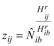
Another stand-level state variable is the mean stem volume (m3), defined as the quotient of the total stand volume and the number of trees. Xue et al. (1999) considered the allometric equation![]() to describe the relationship of mean stand height (H) to mean stem volume (v) and found a good fit in data from Pinus tabulaeformis and Larix principis-rupprechtii stands. I used this interdependence to suggest invariants, quantities that remain unchanged in the absence of disturbances (Table 1), and to derive differential equations estimating the mean volume growth rate in regard with dominant stand height and mean stem volume. The differential equation forms were obtained from the invariants assuming that they were equal to constant and by differentiating both sides of the resultant equations with respect to H. The respective transition functions were derived by equating the invariants for two dominant heights (Table 1). According to the first equation (E1), volume growth depends entirely on the stem volume itself, while the second equation (E2) suggests that the growth rate of mean stem volume depends exponentially on the stand dominant height (Table 1). Alternatively, the third equation (E3) considers both mean stem volume and stand dominant height as predictors of the volume growth rate. From biological viewpoint Equation E1, which predicts volume growth proportional to the mean stem volume (p≈1/3 considering dimensionality of height (m) and volume (m3)), will probably hold true when stands of the same age are compared. For such stands, it is plausible to assume that the bigger mean stem size is a reflection of better site quality and/or wider spacing, which are also prerequisites for faster growth, because of abundant resources and/or reduced competition for them. To conform to the natural laws, however, volume increment cannot increase continuously in time along with the stem size, as suggested by E1 (i.e. the bigger the tree, the faster it grows), because the growth rate of the plants culminates at maturation and then decreases with aging. The transition function based on E1 did not show good fit when tested with the data of Scots pine.
to describe the relationship of mean stand height (H) to mean stem volume (v) and found a good fit in data from Pinus tabulaeformis and Larix principis-rupprechtii stands. I used this interdependence to suggest invariants, quantities that remain unchanged in the absence of disturbances (Table 1), and to derive differential equations estimating the mean volume growth rate in regard with dominant stand height and mean stem volume. The differential equation forms were obtained from the invariants assuming that they were equal to constant and by differentiating both sides of the resultant equations with respect to H. The respective transition functions were derived by equating the invariants for two dominant heights (Table 1). According to the first equation (E1), volume growth depends entirely on the stem volume itself, while the second equation (E2) suggests that the growth rate of mean stem volume depends exponentially on the stand dominant height (Table 1). Alternatively, the third equation (E3) considers both mean stem volume and stand dominant height as predictors of the volume growth rate. From biological viewpoint Equation E1, which predicts volume growth proportional to the mean stem volume (p≈1/3 considering dimensionality of height (m) and volume (m3)), will probably hold true when stands of the same age are compared. For such stands, it is plausible to assume that the bigger mean stem size is a reflection of better site quality and/or wider spacing, which are also prerequisites for faster growth, because of abundant resources and/or reduced competition for them. To conform to the natural laws, however, volume increment cannot increase continuously in time along with the stem size, as suggested by E1 (i.e. the bigger the tree, the faster it grows), because the growth rate of the plants culminates at maturation and then decreases with aging. The transition function based on E1 did not show good fit when tested with the data of Scots pine.
| Table 1. Derivation of mean volume growth sub-model. | |||
| Model | Invariant | Differential equation | Transition function |
| E1 | 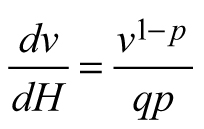 | 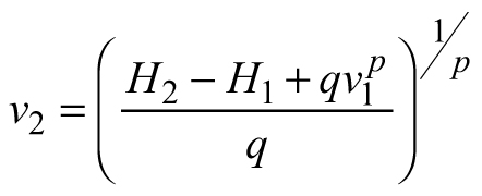 | |
| E2 | 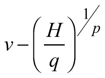 | 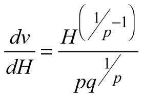 | 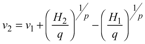 |
| E3 | 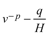 | 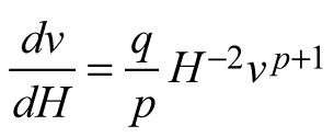 | 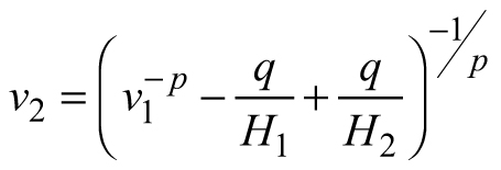 |
| Abbreviations: v − mean stem volume (m3) and H − dominant stand height (m); p, q – global model parameters | |||
Dominant stand height is a good predictor of growth (e.g. Eq. E2), because size is biologically more significant than chronological age as a causal variable, especially in trees, where meristems are constantly renewed (García 2009). However, similarly to model E1, equation E2 also revealed biological inconsistency. According to E2, volume growth is proportional to dominant stand height and no volume growth could be detected, if dominant stand height remains practically unchanged (e.g. at slow height growth), but stand diameter increases. However, since the culmination of the height growth precedes the culmination of the diameter growth, at the time of height growth decrease after its peak stand diameter grows intensively and adds significantly to the stem volume increase. Also, in case of thinning from below, when the dominant stand height is kept constant, model E2 will predict equal volume growth rates for both the thinned and the unthinned stand, which is implausible considering that the trees in the thinned stand have been released from competition and provided with wider growth space.
According to Zeide (1993), the growth equations are composed of two principal components, expansion and decline, and the lack of any of them (as in E1 and E2) makes the model incomplete (Zeide 1993). The expansion component is usually proportional to the size and the decline element to the time variable (Zeide 1993) and the third model derived here (E3) complies with this generalization. When foresters say age they often mean size (García 1994) and stand dominant height can also be viewed as an indicator of stand growth stage, which reflects the interaction between age and site conditions (Stankova and Shibuya 2003). The volume growth predicted by E3 will increase proportionally to the mean stem volume, but this expansion will be controlled by the increase in the dominant height (Table 1). Therefore, when the dominant height growth slows down after its peak, the increase in diameter will contribute to the volume growth by contributing to its expansion factor, the mean stand volume. The dominant stand height will remain the same after thinning from below, but the mean stem volume will be increased. Consequently, the decrease in the stocking due to thinning will be reflected in the increase of the expansion factor of equation E3 and in the volume growth rate, respectively. On the other hand, the mean stand volume of the just-thinned stand might become equal to the mean stand volume of an older stand, of higher dominant stand height. However, their growth rates still will not be equal, because the dominant stand height is inversely related to the growth rate and therefore the younger stand that has been recently released through thinning will grow faster than the older one. Consequently, growth model E3 possesses the ability to discriminate between thinned and unthinned stands and between stands of different development stages. Therefore, the transition function based on E3 will be included as a sub-model in the dynamic growth model for Scots pine plantations.
Considering Eq. 1, stand development stage and site quality are accounted for in the transition function for mean stem volume by the predictor variables H1 and H2. However, volume growth rate might vary even between the stands of the same site index and this specificity is explained primarily by the various levels of stand density resulting in differing competition pressure. Mean stand volume v1 in Eq. E3, which is the quotient of the total stand volume and the number of trees, reflects the level of stand stocking: for stands of same age and site index, smaller value of the mean stem volume and respectively, decreased growth rate, would be ascribed to the larger number of trees. Based on this rationale, which suggests that in general, stand specificity in volume growth is accounted for by the predictor variables and in line with the results by Хue et al. (1999), I assumed that model parameters p and q can be regarded as common to all stands, global model parameters.
2.1.3 Density decrease model
The volume growth model characterizes the average stem size in the stand and is not sufficient to estimate the total yield and merchantable stand volume. A third parameter, which measures the rate of stand stocking, is needed to complete the description and stand density (expressed here as number of trees per hectare) is an appropriate variable to be added to the state vector. The density decrease model can be derived by using a relationship suggested in a study by Vanclay (2009), according to which the mean diameter of trees in pure even-aged forests tends to remain a constant proportion of stand height divided by the logarithm of stand density (N, trees ha–1):
The proposed relationship is a linear regression through the origin of slope β. It may be site-dependent, but it performs better for individual stands than to pooled data and once a stand has established a trajectory, it tends to maintain the same trajectory for a long time (Vanclay 2009). Consequently, the slope β can be viewed as a stand-specific constant. If we apply again the relationship, known as the allometric equation, to relate mean stand diameter DBH to stand dominant height H, i.e. DBH = aHb, Eq. 2 will be rewritten as:

Equation 3 proposes an exponential relationship between stand density and dominant stand height raised to a power. Subtraction of a constant value of 1.3 from the stand height has been introduced in Eq. 2 to ensure that the trend passes through the origin for trees approaching breast height. This requirement no longer holds for the density decrease model of Eq. 3, which describes a trend of reduction in the tree number with the dominant height increase. Consequently, the multiplier (H – 1.3) in Eq. 3 can be replaced, for convenience, by the power of height Hc, and the resultant new formulation for the density decrease function is:
where ![]() obtains positive values (β, a > 0) and r = c – b is a global model parameter. Vanclay (2009) showed with extended set of data the robustness of his relationship (Eq. 2) and the stability of the specific constant β, which manifested time-invariance and invariance with thinnings. Parameter φ of Eq. 4 is a quotient of Vanclay’s specific constant β and a global constant and consequently it is implicitly derived as a local (stand-specific) parameter. To derive the algebraic difference equation (ADA) form of Eq. 4, it was first solved for the local parameter φ,
obtains positive values (β, a > 0) and r = c – b is a global model parameter. Vanclay (2009) showed with extended set of data the robustness of his relationship (Eq. 2) and the stability of the specific constant β, which manifested time-invariance and invariance with thinnings. Parameter φ of Eq. 4 is a quotient of Vanclay’s specific constant β and a global constant and consequently it is implicitly derived as a local (stand-specific) parameter. To derive the algebraic difference equation (ADA) form of Eq. 4, it was first solved for the local parameter φ,

then its value was equated for two points on the density decrease curve ![]() and finally the projected stand density N2 was expressed to obtain a dynamic equation for the stand density decrease:
and finally the projected stand density N2 was expressed to obtain a dynamic equation for the stand density decrease:

where Nj (j = 1, 2) is stand density (trees.ha–1) and Hj is dominant stand height (m) of the j-th measurement. Equation 6 was included as a transition function for the density decrease in the dynamic whole-stand model.
2.1.4 Mean volume prediction function
As already shown, the survival model can be easily initialized from any pair of height-density measurements, which provide estimate of the stand-specific constant and define the density decrease course for the stand. The volume projection function can be started from bare land by setting the initial conditions for unthinned stand H1 = H0 = 0, v1 = v0 = 0in Eq. E3 thus obtaining:

When we have to apply the model to a managed stand, however, we sometimes do not know the parameters of the remaining stand after the thinning, i.e. we do not have the information needed to initialize the volume projection model. Consequently, a mean stem volume prediction function is needed, which would recover its value at any time from the readily available stand information, e.g. dominant stand height and tree number. It has been asserted (Barrio-Anta et al. 2006; Castedo-Dorado et al. 2007b) that to assure compatibility between the projection (e.g. Eq. E3) and the initialization functions, they should be related by the same base equation (e.g. Eq. 7). Since Eq. 7 estimates the mean stem volume of an unthinned stand, the mean volume of the same stand at the same growth stage (i.e. dominant stand height) is expected to be higher when thinned, i.e. when the stand stocking has been decreased. Consequently, the mean stem volume increase, relative to the unmanaged stand, can be presumed inversely proportional to the stand stocking. Therefore, a prediction function of the form 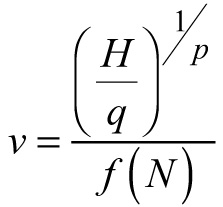 can be suggested to recover the value of the mean stem volume from the stand dominant height and density. Several formulations for f (N) were tested, e.g. s′Nm, s′ln(N)m and their derivatives for fixed values of m (e.g. m = 1, 3/2, 2, 3). The model, which was successfully fitted to the Scots pine data and was chosen as a stem volume prediction equation obtained the form:
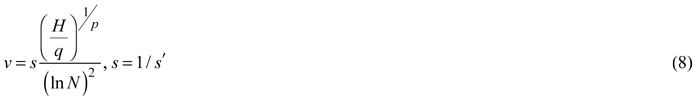
The tentative and rather simplified nature of Eq. 8 implies that it should be used only when it is indispensable for the model application.
2.2 Data set and data assessment
The model was tested with a data set of stand-level variables (Table 2) collected in 79 permanent sample plots of size 150–2000 m2 established in Scots pine plantations in Bulgaria at 450–1600 m a.s.l. The plots have been measured 2 to 5 times and the data set included 239 plot measurements in total. The data were compiled from several sources. Thirty-five of the sample plots have been used to develop growth and yield tables for Scots pine plantations (Krastanov et al. 1980). These have been remeasured once or twice at 2 to 6 year intervals and have been exposed to different thinning treatments and thinning intensities. Two of the experimental plots are established in Scots pine plantations against erosion and have been re-measured once: the first one after two years and the other one after three years (Marinov 2008). Each of the remaining plots is presented in two variants, one of which is assigned for silvicultural treatment and the other is a control plot (42 plots in total). These are permanent sample plots established for growth and yield studies by the forest enterprises responsible for development of forest management plans, and they have been measured two to four times at 9 to 12-year intervals. These data were available from the current and the archived forest management plans of the local forest management units. The plot dominant height was estimated from the experimental mean plot height by the relationship established by Stankova et al. (2006). Data obtained before and after the thinning of the treated plots were considered as distinct time series thus yielding 98 data series from 79 plots. This was because silvicultural treatments such as thinning cause an instantaneous change in the state variables of the stand and the system must therefore estimate the trajectories starting from the new state after thinning (Castedo-Dorado et al. 2007a).
| Table 2. Description of the data set. | ||||
| Stand variable | Mean | Standard deviation | Minimum | Maximum |
| DBH (cm) | 17.7 | 6.0 | 5.6 | 34.7 |
| N (trees ha–1) | 2270 | 1862 | 393 | 9305 |
| H (m) | 16.3 | 5.0 | 6.3 | 32.5 |
| Age (years) | 38 | 14 | 12 | 80 |
| v (m3) | 0.260 | 0.218 | 0.011 | 1.257 |
| y (m3 ha–1) | 340.7 | 144.6 | 61.4 | 723.4 |
| Abbreviations: DBH – diameter at breast height; H − dominant stand height; N – stand density; v – mean stem volume; y – total stand volume | ||||
The data set used for site index model derivation and parameterization was a subset of the data used in the current study and included plots that have not been thinned, or have been exposed to light thinnings from below. I applied Eq. 1 also to calculate the site indices for the entire data set used to develop the dynamic whole-stand model in order to assess graphically their quality, as suggested by Vanclay et al. (1995) (Fig. 1). Examination charts showed that the data span plantation ages from 12 to 80 years, allocated between stands of three different site index classes (Fig. 1a). Young plantations of high site indices are somewhat underrepresented (Fig. 1a, c) and site index extremes are not included in the data set (Fig. 1c); however, the data for both low- and highly-stocked stands are found at different site quality conditions (Fig. 1a), and the predominating age-site quality range is well represented (Fig. 1c). The inclusion of plots in unthinned plantations provided observations from overstocked populations, while the availability of plots in managed stands enabled representation of a range of stocking levels and types of silvicultural manipulation during the period of intensive management (Fig. 1b). As a result of the data appraisal, I concluded that the available data are of sufficient quality for development of a dynamic growth model, although it must be borne in mind that the relatively small total number of sample plots and data heterogeneity (regarding their origin, re-measurement frequencies and intervals) may obscure the application of more sophisticated model formulations.
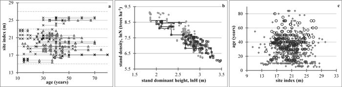
Fig. 1. Data examination charts. a – Stand age-site index data range of this study. Basal area values below (×) and above (▲) average are indicated. Solid lines connect measurements of the same plot, for site index averaged per plot. Dotted gridlines delimit 4m-site index classes. b – Dominant stand height-stand density data range. Site index values below (●) and above (□) average are indicated. Thinning trajectories for some of the managed plots are represented by solid lines; c – Site index-stand age data comparison between the permanent sample plots of this study (◌) and temporary sample plot data (♦). Site index model by Stankova and Diéguez-Aranda (2012) for reference age 50 years and temporary sample plots data from Stankova and Shibuya (2007) are used. View larger in new window/tab.
2.3 Model examination
The transition functions corresponding to Eqs. 6 and E3 were fitted using a Base-Height Invariant (BHI) dummy variable approach (Stankova and Diéguez-Aranda 2013), which is analogous to the Base-Age Invariant (BAI) dummy variable approach proposed by Cieszewski et al. (2000) and where dominant height is used for projection instead of age. The implementation of this method requires fitting the difference equations in the following manner:
the density decrease model as:
the mean volume model as:
where Nij and vij are the estimated response variables stand density (trees ha–1) and mean stem volume (m3) of data series i (data obtained before and after the thinning of the treated plots were considered as distinct data series, i.e. the number of the plots does not equal the number of the data series) at measurement occasion j, Hij is the predictor variable stand dominant height of data series i at occasion j, pi are dummy variables of value 1 for data series i and 0otherwise, Hib is base dominant height (corresponding to the base age in the original method) arbitrarily assigned to each data series i, Nib is the value of density (trees ha–1) corresponding to Hib and vib is the value of mean stem volume (m3) at Hib. Stand density and mean stem volume corresponding to Hib (on the right-hand side of Eqs. 9 and 10) are estimated as stand-specific, local model parameters![]() and
and![]() (where
(where![]() is predicted stand density corresponding to Hib, and
is predicted stand density corresponding to Hib, and![]() is predicted mean stem volume at Hib), while the respective experimentally measured figures provide only initial values for fast convergence. Consequently, the variable values corresponding to the base dominant heights are also allowed to vary (i.e. produce residuals) along with the response variables and are estimated for all stands simultaneously with the global model parameters. This methodological procedure shows similarity to the mixed-effects modeling (Cieszewski et al. 2000) and assures fitting the curve to the observed trend in the data rather than forcing the model through any given measurement.
is predicted mean stem volume at Hib), while the respective experimentally measured figures provide only initial values for fast convergence. Consequently, the variable values corresponding to the base dominant heights are also allowed to vary (i.e. produce residuals) along with the response variables and are estimated for all stands simultaneously with the global model parameters. This methodological procedure shows similarity to the mixed-effects modeling (Cieszewski et al. 2000) and assures fitting the curve to the observed trend in the data rather than forcing the model through any given measurement.
The total stand volume can be obtained as the product of the mean stem volume projected with the dominant height growth and the number of trees survived at the end of the growth period. The endogenous (response) variable stand density was substituted by an appropriate formulation, derived from Eq. 6, on the right-hand side of Eq. 8 and in the total stand volume equation, and the estimated projected mean volume was presented in the total stand volume equation by the right-hand expression of Eq. E3. Such reformulation places the endogenous variables on the left-hand side of the equations only, which allowed their simultaneous fitting by Nonlinear Seemingly Unrelated Regression (NSUR) to account for cross-equation correlations. The final whole-stand dynamic growth model for predicting and projecting the principal stand growth variables was composed from the following four sub-models:
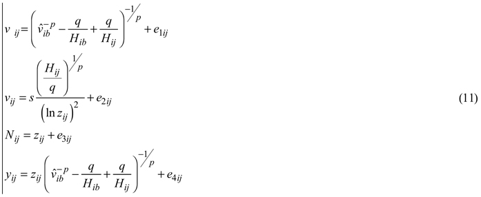
where
In Eqs. 11 yij is the estimated response variable total stand volume (m3ha–1) of data series i at measurement occasion j, p, q, r and s are global model parameters and e1ij, e2ij, e3ij, e4ij are random errors. The first and second sub-models of Eqs. 11, which stand for the same response variable, were presented and fitted in general equation form (SAS Institute Inc. 2013) to allow their concomitant estimation.
Plots of residuals against lag-residuals were examined and did not reveal the presence of autocorrelated errors (Fig. 2), which could have been expected, because the utilized forest stand data are constituted of a multiplicity of concurrent, relatively short time series. However, graphical and analytical indications of heteroscedasticity (e.g. Fig. 4) imposed the application of Heteroscedasticity-Consistent Covariance Matrix Estimator (HCCME) to ensure the efficiency of the regression estimates (Long and Ervin 2000). The goodness-of-fit of the whole-stand dynamic growth system was evaluated by the adjusted coefficients of determination, the root mean squared errors, the absolute and relative biases of the principal model equations and by examining the plots of observed against predicted values. The simultaneous equation fitting was programmed using the SAS/ETS® MODEL procedure (SAS Institute Inc. 2013) and all statistical analyses were performed employing the SAS software.
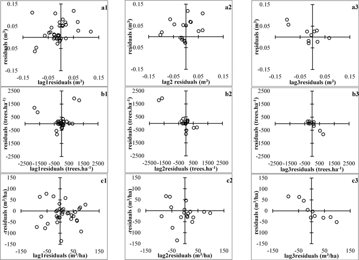
Fig. 2. Plots of residuals vs lag−residuals. a1 to a3 – mean stem volume, m3; b1 to b3 – stand density, ha-1; c1 to c3 – total stand volume m3/ha. View larger in new window/tab.
2.4 Model validation
Plausibility and applicability of the whole-stand dynamic model were examined and validated in two directions. First, the accuracy of model predictions was assessed through estimation of the tolerance intervals for the relative errors. This particular interval test statistic was chosen, because it reveals the worst possible prediction scenarios, i.e. it shows, with a high level of certainty (e.g. 99%), the range of the possible deviations from the reality, as relative to the values of the variables of interest, for the bulk (e.g. 50–95%) of the error distribution. Next, model unbiasedness regarding its application to thinned and unthinned stands was assured.
2.4.1 Prediction errors of the future observations
The tolerance intervals were estimated with a data set constructed from the available parameterization data set specifically for this validation. All possible predictor-predicted pairs of measurements (both forward and backward in time) were considered, and the resultant data set for validation included 504 pairs of observations in total. Tolerance intervals (TI) for the relative errors in 50, 75 and 95% of the future observations with 99% probability were estimated:
where B is the relative bias, S is the standard deviation of the errors, the function g(1–γ, n, 1–α) is the tolerance factor tabulated for specified values of n, α and γ and provides that the estimated interval will contain at least (1–γ)100 percent of the future error distribution with probability (1–α).
2.4.2 Model consistency regarding thinnings
Abrupt alteration of the principal stand characteristics during thinning can affect growth dynamics in such a way that, growth underestimation for the unthinned and its overestimation for the thinned stands can be induced (Pienaar and Shiver 1986; Barrio-Anta et al. 2006; Castedo-Dorado et al. 2007b), when developing a model for combined data from both unthinned and thinned stands. To account for the possible treatment effect, both transition functions (Eqs. 6 and E3) derived within this study were initially assessed after expanding of each of the global parameters (r and, p and q, respectively), by inclusion of a dummy variable accounting for the treatment effect as: a + Itb, where a is the global parameter, It is the dummy categorical variable for considering the silvicultural treatment and obtains value 0for unthinned and value 1 for just-thinned stands and b is the parameter associated with the respective dummy variable. Additionally, the invariance of the stand-specific parameter φ of the density decrease model was validated. Upon estimation of the global model parameter r, it was substituted into Eq. 5 and the stand-specific constant φ was calculated for each pair (Hij – Nij) of height-density measurements. Stability of the parameter estimates was then evaluated using two test statistics: coefficient of variation (%) and percent relative standard error PRSE(%) = 100×(SE/|φ|), where SE is the standard error. These test-statistics were calculated by data series and by plots to assess both the time-invariance and the thinning-invariance of the
3 Results
The mean volume projection function (E3) was fitted with either or both global parameters accounting for the treatment effect, but none of them produced significantly different from zero dummy-variable-associated parameter estimates. The density decrease model (Eq. 6), on the other hand, did not produce significant values for the expanded model parameters, when Heteroscedasticity-Consistent Covariance Matrix Estimator was applied to assess the efficiency of the estimates. The goodness-of-fit statistics for the whole-stand dynamic growth system, composed of the four simultaneously evaluated regression equations (Eqs. 11), are shown in Table 3. Fig.3 presents plots of experimental against estimated values of the dependent model variables, along with the results of the simultaneous F test for slope equal to one and zero intercept of the linear regressions relating them (Figs. 3c–3f), and illustrates the projected time trajectories of stand density and mean volume (Figs. 3a, b). Both graphs and tests demonstrated a lack of bias of the regression equations, as inferred from the small and insignificantly different from zero absolute and relative biases (Table 3) and also from the accepted hypotheses for linear regression through the origin between observed and predicted values for all stand growth variables. All dynamic relationships attained high coefficients of determination (between 0.919 and 0.948) and small root mean squared errors (Table 3), which together with the fitted trends in stocking and mean volume, illustrated on Figs 3a, b, confirmed that the growth processes are adequately described by the projection functions.
| Table 3. Goodness - of - fit statistics for the whole-stand dynamic model. | |||||||
| Global model parameters | Regression estimation a | ||||||
| Parameter: Estimate | p: 0.4740 | Dependent variable | Adj. R2 | RMSE | Bias b | Relative bias (%) b | |
| ASE HCCME | 0.0207 0.0556 | ||||||
| Parameter: Estimate | q: 37.934 | Stand density | 0.948 | 403 | –11 | –0.37 | |
| ASE HCCME | 2.9410 9.1053 | ||||||
| Mean stem volume (projected) | 0.931 | 0.0460 | –0.0002 | –2.42 | |||
| Parameter: Estimate | r: –0.0945 | ||||||
| ASE HCCME | 0.0067 0.0402 | Mean stem volume (predicted) | 0.740 | 0.0893 | 0.0034 | –10.68 | |
| Parameter: Estimate | s: 69.279 | ||||||
| ASE HCCME | 8.6749 27.317 | Total stand volume | 0.919 | 41.81 | –0.480 | –1.89 | |
| Abbreviations: ASE – Asymptotic Standard Error; HCCME – Heteroscedasticity - Consistent Covariance Matrix Estimator; Adj. R2 – adjusted coefficient of determination; RMSE – Root Mean Square Error. a Total number of observations N = 239. b The absolute and relative biases for all estimated stand variables are not significantly different from zero. | |||||||
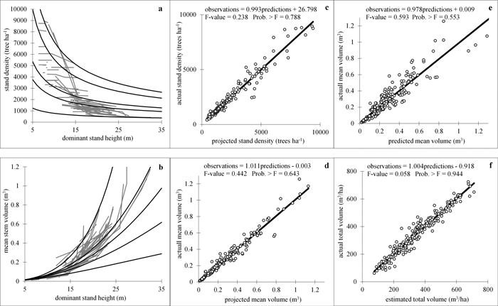
Fig. 3. Goodness-of-fit and prediction charts. a, b − density decrease (a) and volume growth (b) models fitted to the experimental data. Fitted curves for five data series comprising the data range are shown; c, d actual vs. projected values: stand density (c) and mean stem volume (d); e − actual vs. predicted mean stem volume; f − actual vs. estimated total stand volume. Linear regressions of observed against estimated variable values are fitted and the results from simultaneous F-test for line slope equals 1 and zero intercept (Gadow and Hui 1999) are shown in the plots. View larger in new window/tab.
The mortality rate model (Eq. 6), when evaluated in the expanded-parameter form, suggested increased value of the exponent r for the treated stands, leading to respectively higher survival rates as compared to the unthinned stands of the same starting densities. The same tendency was indicated also by the residual plot (Fig. 4c) where the projected stocking rates of the higher-density thinned stands seemed under-evaluated. Analysis of the stand specific parameter φ of the density decrease model, however, showed that its variation was insignificant both within the data series and within the plots, which included thinned and unthinned data series. Indeed, its coefficient of variation ranged from 0.02 to 5.08% between data series and from 0.02 to 6.52% between plots, while the percent relative standard error (PRSE) had range of 0.01–2.93% for both, data series and plots. These test statistics not only confirmed that the specific parameter is a constant, irrespective of the growth stage and the management background of the stand, but also revealed that, at the level of each population in particular the possible underestimation of the projected density of the thinned stand is relatively negligible (Fig. 4c). No trends to biased estimates of mean stem predicted and projected volume and total stand volume were noticeable with respect to treatment from the plots of predicted values vs. residuals (Figs. 4a, b, d).
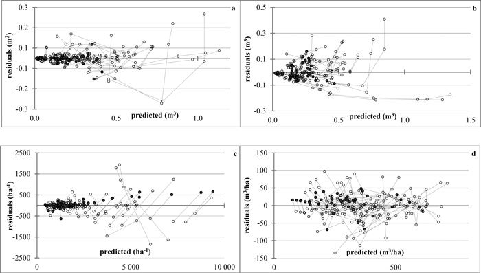
Fig. 4. Plots of residuals vs. predicted values. a – projected mean stem volume; b – predicted mean stem volume; c – stand density; d – total stand volume. The lines connect the residuals (◌) by data series, the symbol ● denoting values of just-thinned plots. View larger in new window/tab.
The error terms calculated for the data set constructed specifically for validation deviated from the normal distribution, and 10% trimmed means and jackknife standard deviations were therefore used to estimate the tolerance intervals (Rauscher 1986). The error ranges for volume and density revealed acceptable values for 3/4 of the future observations (Table 4). It can be concluded with 99% probability that in 75% of the future observations, the projected mean stem volume will exceed the true values of this variable by less than 30%. Stand density and total volume prediction errors amounted to less than 35% for 75% of the future observations with 99% certainty (Table 4).
| Table 4. Validation test statistics of the whole-stand dynamic model. | ||||||
| Dependent variable | Tolerance intervals (TI) for the relative errors 1 – α = 99% probability for the future errors | |||||
| 1 – γ = 50% | 1 – γ = 75% | 1 – γ = 95% | ||||
| of future observations | ||||||
| Stand density | –19.6 | 17.6 | –32.7 | 30.7 | –54.9 | 53.0 |
| Projected mean stem volume | –17.4 | 16.4 | –29.4 | 28.4 | –49.7 | 48.7 |
| Predicted mean stem volume | –33.4 | 12.9 | –49.8 | 29.2 | –77.5 | 57.0 |
| Total stand volume | –18.8 | 19.2 | –32.2 | 32.6 | –54.9 | 55.4 |
The mean volume prediction function showed poorer fit than the other three sub-models, as seen from the regression goodness-of-fit statistics and from the tolerance intervals for the errors in future observations (Tables 3 and 4). This function, however, is of auxiliary nature and due to the unbiased estimates that it produces, it can assist the whole-stand dynamic model application when needed.
In summary, given the state of the stand at present, the following sequence of equations can be solved to predict its state at a desired future stage:

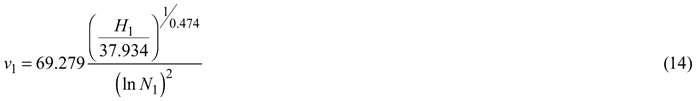


where Eqs. 13 and 14 are optional.
4 Discussion
The model derived here is based on the state-space approach, which has already been applied to develop stand-level dynamic growth models for Scots pine and Radiata pine plantations, natural birch and oak stands in north-western Spain (Diéguez-Aranda et al. 2006; Castedo-Dorado et al. 2007a; Gómez-García et al., 2010, 2015), natural stands of European beech in Switzerland (Álvarez-González et al. 2010), interior spruce stands in British Columbia (García 2011), loblolly pine plantations in the USA (García et al. 2011), trembling aspen in Western Canada (García 2013a), teak plantations in India (Tewari et al. 2014). These preceding models can be classified into two groups, according to the variables included in the state vector to describe the stand and used for future projections through the transition functions. In the dynamic growth models developed in Europe, the initial conditions at any point in time are defined by three state variables – number of trees per hectare, stand basal area and dominant height, which all are projected in time, while the models of the second group (by García 2011; García et al. 2011; García 2013a and Tewari at al. 2014) include four state variables (top height, trees per hectare, basal area and a measure of stand closure), of which dominant height growth is projected with stand age, while the other state variables are projected with respect to dominant height growth. This study proposed a dynamic growth model based on three state variables, two of which − dominant height and trees per hectare – have already been used in the earlier models, while the mean stem volume was proposed here as a third state variable and along with stand density, measured as tree number, was projected in regard to the temporal change of stand dominant height.
The widely used growth functions by Bertalanffy-Richards, Lundqvist-Korf and Hossfeld are commonly utilised in the transition functions for projecting dominant height growth in time. The transition function for dominant height in the models of García (García 2011; García et al. 2011; García 2013a) is derived from the base differential equation of the respective growth function (e.g. Bertalanffy-Richards in most cases), while the rest of the authors preferred to use the techniques for dynamic equation derivation known in forestry as the Algebraic Difference Approach (ADA; Bailey and Clutter, 1974) or its generalization (GADA; Cieszewski 2003), as it was done also in this study. A dynamic, anamorphic, base-age invariant site index model was used as a transition function for the dominant height of the Scots pine plantations in Bulgaria since some data limitations (relatively small number of sample plots, indirect estimation of the dominant stand height, lack of data from stem analysis) has prevented development of more flexible and biologically adequate GADA formulation (Stankova and Diéguez-Aranda 2012). However, the reliability of Eq. 1 has been revealed through its high goodness-of-fit and accuracy estimates as well as by its manifested superiority to the currently applied site index tables for Scots pine plantations that have limited applicability, because of their narrow age-height range and poor fit to the actual growth trajectories (Stankova and Diéguez-Aranda 2012). Monserud (1984) considered specifying site quality models by habitat types, while Colff and Kimberley (2013) derived an improved, national height-age model for Radiata pine in New Zealand, by expressing the slope parameter of the model as a function of elevation and latitude, which together account for temperature. According to Bravo-Oviedo et al. (2008) global accuracy for specific regions is greatly improved if climatic models are applied when climatic or edaphic variability is high (Bravo-Oviedo et al. 2008). Consequently, in spite of the undoubted flexibility of the site quality curves manifesting polymorphism and/or multiple asymptotes (e.g. those derived by ADA and GADA), the development of a site index model that accounts for regional, habitat and environmental differences can be considered as a subject of future research, because of the variability in forest sites.
The state variable stand density (expressed as number of trees per hectare) was projected with age change in the models by Castedo-Dorado et al. (2007a), Álvarez-González et al. (2010) and Gómez-García et al. (2010, 2015), and the density decrease function accounted also for the influence of site quality in the model for Scots pine from north-western Spain by Diéguez-Aranda et al. (2006). The rest of the dynamic models employed a site-independent relationship for the mortality relative to height growth derived by García (2009). Similarly, by utilizing a relationship by Vanclay (2009) and applying the algebraic difference approach (ADA) for developing of dynamic equations, I derived a dominant height-dependent transition function for stand stocking. The base integral equation form of the new model (Eq. 4) proposes an exponential relationship between the number of trees and dominant stand height raised to a power, describes a reverse sigmoid density decrease pattern and is consistent with the requirement formulated by Clutter et al. (1983) for asymptotic zero limit of stand density at very advanced growth stage. In addition, stand-specific values of asymptotic stand density at the initial growth stage (if designated by stand height H = 1 m) equal to exp(φ) are inferred from the model formulation.
The stand basal area was the third principal state variable in the preceding dynamic growth systems, which apply the state-space modelling approach. It has been directly projected in time in the models for Scots pine and Radiata pine plantations from north-western Spain and for beech stands from Switzerland (Diéguez-Aranda et al. 2006; Castedo-Dorado et al. 2007a; Álvarez-González et al. 2010), while the models for Downy birch and English oak by Gómez-García et al. (2010, 2015) incorporated also dominant stand height and tree number as predictor variables. Álvarez-González et al. (2010) considered the thinning effect on the basal area growth by discriminating parametrically the basal area transition functions for thinned and unthinned stands. García (2011), on the other hand, who preferred to project stand basal area indirectly through its product with stand dominant height, included site occupancy as a forth state variable to account for the increment reduction, specific for the young or recently thinned stands that still do not fully occupy the available growth space. In the rationale provided in the derivation of mean stem volume transition function, I showed how the thinning effect was considered in this study through the choice of invariant and differential equation, to suggest biologically sound description of volume increment relative to height growth. As revealed also by the validation, no significant differences between the parameter values of the volume transition function were found for the unthinned and just-thinned plantations, which confirms that the thinning effect was actually built into the model. Decrease in the stocking due to thinning from below is reflected in increased mean stem volume and, through Eq. E3, in accelerated volume growth rate of the retained plants. A thinning from above, on the other hand, would reduce the average stem volume of the remaining stand, but will also decrease the dominant stand height. The values of the exponents of Eq. E3 (around 1.5 in the numerator and 2 in the denominator) suggest that the change in the reduction factor (i.e. height) will have more pronounced effect on the volume growth than the alteration of the expansion component (i.e. stem volume). Consequently, this type of management treatment will also result in increased volume growth. The younger stand that has been recently released through thinning, on the other hand, will grow faster than an older stand of the same mean stem volume due to its smaller stand dominant height, playing the role of a reduction factor in Eq. E3. Similar to the studies on development of a basal area growth system by Barrio-Anta et al. (2006), Diéguez-Aranda et al. (2006), Castedo-Dorado et al. (2007a, b) and Gómez-García et al. (2010, 2015), the mean stem volume growth system here was composed by two sub-modules: one for mean stand volume initialization and another for its projection. It was developed using the same base equation to assure the concordance of the component models, with the objective to provide initial condition value of mean volume when it is not obtainable from common forest inventory data. The mean stem volume and stand stocking transition functions were fitted simultaneously with the total stand volume estimation to ascertain model compatibility and to strengthen the predictive power of the model.
Longitudinal data are rarely ample and usually far from ideal for model development. García (2011) recommended sound biological basis of the model and low number of estimated model parameters as a means to cope with scarcity and limited representativeness of the data. To adapt the more complicated model formulations for basal area growth to their data, García et al. (2011), García (2013a) and Tewari et al. (2014) applied restrictions to particular model parameters by fixing their values to logically derived constants. This was done to achieve convergence and reasonable parameter estimates. Parsimony of the formulated projection models was the principal approach used in this study to deal with the limited amount of repeated measurements data and it was pursued as a balance between biological plausibility and simplicity.
The growth and yield tables currently implemented in Bulgarian forest inventory and management can be classified as second-generation whole-stand models (Pretzsch 2009). They present the most important average and cumulative stand characteristics, according to established silvicultural prescriptions, in homogeneous even-aged managed “normal” stands, usually every 5 years (Nedyalkov et al. 1983). The use of growth and yield tables is a robust approach to growth and yield prediction but it is severely constrained by the need to follow a standard production regime (Pretzsch 2009). In many situations where decision support is needed, a growth model is required to explore different harvesting and management options (Vanclay 2010). Scarcity of repeated-measurements data, however, often prevents the use of more elaborate modelling approaches. The dynamic whole-stand growth model derived here belongs to the advanced-generation whole-stand models, provides information about the current values of the main stand characteristics and projects stand development for a broad spectrum of potential management alternatives.
A whole-stand dynamic growth model, which constitutes a simple and robust system of state variables and transition functions and enables easy and reliable description and projection of growth and yield of even-aged forest stands, was derived. The model is parsimonious, which allows its estimation when longitudinal data are scarce, and can be incorporated into a computer program (simulator) and disseminated for practical implementation.
Acknowledgements
I wish to thank the Forest Research Institute of the Bulgarian Academy of Sciences, which made available, through a research report in its possession, some of the data used in this study, Prof. Ivan Marinov for the data from the experimental plots established in plantations against erosion, Assoc. Prof. Ulises Diéguez-Aranda and Dr. Esteban Gómez-García for their advice on the simultaneous equation fitting and to Prof. Oscar García for his valuable guidance during the derivation of this model.
References
Álvarez-González J.G., Zingg A., Gadow K.v. (2010) Estimating growth in beech forests: a study based on long term experiments in Switzerland. Annals of Forest Science 67: 307. http://dx.doi.org/10.1051/forest/2009113.
Assmann E. (1970) The principles of forest yield study. Pergamon Press, Oxford. p. 160.
Barrio-Anta M., Castedo-Dorado F., Diéguez-Aranda U., Álvarez-González J.G., Parresol B.R., Rodríguez-Soalleiro R. (2006). Development of a basal area growth system for maritime pine in northwestern Spain using the generalized algebraic difference approach. Canadian Journal of Forest Research 36: 1461–1474. http://dx.doi.org/10.1139/X06-028.
Bailey R.L., Clutter J.L. (1974). Base-age invariant polymorphic site curves. Forest Science 20: 155–159.
Bravo-Oviedo A., Tomé M., Bravo F., Montero G., Río M. d. (2008) Dominant height growth equations including site attributes in the generalized algebraic difference approach. Canadian Journal of Forest Research 38: 2348–2358. http://dx.doi.org/10.1139/X08-077.
Burkhart H.E., Tomé M. (2012). Modelling forest trees and stands. Springer Sience+Business Media, Dordrecht. p. 237–260. http://dx.doi.org/10.1007/978-90-481-3170-9.
Castedo-Dorado F., Diéguez-Aranda U., Álvarez-González J.G. (2007a). A growth model for Pinus radiata D. Don stands in northwestern Spain. Annals of Forest Science 64: 453–465. http://dx.doi.org/10.1051/forest:2007023.
Castedo-Dorado F., Diéguez-Aranda U., Barrio-Anta M., Álvarez-González J.G. (2007b). Modelling stand basal area growth for radiata pine plantations in Northwestern Spain using the GADA. Annals of Forest Science 64: 609–619. http://dx.doi.org/10.1051/forest:2007039.
Cieszewski C.J. (2003). Developing a well-behaved dynamic site equation using a modified Hossfeld IV function Y3 = (axm)/ (c + xm_1), a simplified mixed-model and scant subalpine fir data. Forest Science 49: 539–554.
Cieszewski C.J., Harrison M., Martin S.W. (2000). Practical methods for estimating non-biased parameters in self-referencing growth and yield models. University of Georgia PMRC-TR 7.
Clutter J.L., Fortson J.C., Pienaar L.V., Brister G.H., Bailey R.L. (1983). Timber management: a quantitative approach. John Wiley & Sons, NY, USA. p. 92,132.
Colff M.vd, Kimberley M.O. (2013). A National height-age model for Pinus radiata in New Zealand. New Zealand Journal of Forest Science 43: 4. http://www.nzjforestryscience.com/content/43/1/4. [Cited 29 May 2015].
Diéguez-Aranda U., Castedo-Dorado F., Álvarez-González J.G., Rojo A. (2006). Dynamic growth model for Scots pine (Pinus sylvestris L.) plantations in Galicia (north-western Spain). Ecological Modelling 191: 225–242. http://dx.doi.org/10.1016/j.ecolmodel.2005.04.026.
Gadow K. v., Hui G. (1999). Modelling forest development. Kluwer Academic Publishers, Dordrecht. p. 49, 189. http://dx.doi.org/10.1007/978-94-011-4816-0.
García O. (1988). Growth modelling - a (re)view. New Zealand Forestry 33(3): 14–17.
García O. (1994). The state-space approach in growth modeling. Canadian Journal of Forest Research 24: 1894–1903. http://dx.doi.org/10.1139/x94-244.
García O. (2009). A simple and effective forest stand mortality model. Mathematical and Computational Forestry & Natural-Resource Sciences 1(1): 1–9.
García O. (2011). A parsimonious dynamic stand model for interior spruce in British Columbia. Forest Science 57(4): 265–280.
García O. (2013a). Building a dynamic growth model for trembling aspen in western Canada without age data. Canadian Journal of Forest Research 43(3): 256–265. http://dx.doi.org/10.1139/cjfr-2012-0366.
García O. (2013b). Forest stands as dynamical systems: an introduction. Modern Applied Science 7(5): 32–38. http://dx.doi.org/10.5539/mas.v7n5p32.
García O., Burkhart H.E., Amateis R.L. (2011). A biologically-consistent stand growth model for loblolly pine in the Piedmont physiographic region, USA. Forest Ecology and Management 262: 2035–2041. http://dx.doi.org/10.1016/j.foreco.2011.08.047.
Gómez-García E., Crecente-Campo F., Stankova T., Rojo A., Diéguez-Aranda U. (2010). Dynamic growth model for Birch stands in northwestern Spain. Forestry Ideas 16(2): 211–220.
Gómez-García E., Crecente-Campo F., Barrio-Anta M., Diéguez-Aranda U. (2015). A disaggregated dynamic model for predicting volume, biomass and carbon stocks in even-aged pedunculate oak stands in Galicia (NW Spain). European Journal of Forest Research 134: 569–583. http://dx.doi.org/10.1007/s10342-015-0873-3.
Hasenauer H. (Ed.) (2006). Sustainable forest management. Growth models for Europe. Springer, Berlin-Heidelberg. p. 5.
Huxley J.S. (1972). Problems of relative growth. 2nd edition. Dover Publications Inc, New York. p. 6–13.
Krastanov K., Belyakov P., Shikov K. (1980). Dependencies in the structure, growth and productivity of the Scots pine plantations and thinning activities in them. Available from the Forest Research Institute of Bulgarian Academy of Sciences, Sofia Research report. [In Bulgarian].
Long J.S., Ervin L.H. (2000). Using heteroscedasticity consistent standard errors in the linear regression models. American Statistician 54(3): 217–224.
Marinov I. (2008). Investigation and evaluation of erosion in some regions of South-western Bulgaria. DSci thesis. Department of Ecology, Forest Research Institute of Bulgarian Academy of Sciences, Sofia. [In Bulgarian].
Monserud R.A. (1984). Height growth and site index curves for inland Douglas-fir based on stem analysis data and forest habitat type. Forest Science 4: 943–965.
Nedyalkov S., Rashkov R, Tashkov R. (1983). Reference book in dendrobiometry. Zemizdat, Sofia. p. 305–549. [In Bulgarian].
Pienaar L.V., Shiver B.D. (1986). Basal area prediction and projection equations for pine plantations. Forest Science 32(3): 626–633.
Pretzsch H. (2009). Forest dynamics, growth and yield. from measurement to model. Springer-Verlag, Berlin Heidelberg. p. 387–389, 432–445.
Rauscher H.M. (1986). The microcomputer scientific software series 4: testing prediction accuracy. North Central Forest Experiment Station, U.S. Department of Agriculture - Forest Service, Minnesota. U.S. For. Serv. Gen. Tech. Rep. NC-107.
SAS Institute Inc. (2013). SAS/ETS® 12.3 user’s guide. SAS Institute Inc, Cary, NC. p. 1015–1335.
Stankova T., Diéguez-Aranda U. (2012). A tentative dynamic site index model for Scots pine (Pinus sylvestris L.) plantations in Bulgaria. Silva Balcanica 13(1): 5−19.
Stankova T., Diéguez-Aranda U. (2013). Simple and reliable models of density decrease with dominant height growth for even-aged natural stands and plantations. Annals of Forest Science 70(6): 621–630. http://dx.doi.org/10.1007/s13595-013-0303-y.
Stankova T., Shibuya M. (2003). Adaptation of Hagihara’s competition-density theory to natural birch stands. Forest Ecology and Management 186(1–3): 7−20. http://dx.doi.org/10.1016/S0378-1127(03)00260-3.
Stankova T., Shibuya M. (2007). Stand Density Control Diagrams for Scots pine and Austrian black pine plantations in Bulgaria. New Forests 34(2): 123–141. http://dx.doi.org/10.1007/s11056-007-9043-x.
Stankova T., Stankov H., Shibuya M. (2006). Mean-dominant height relationships for Scotch pine and Austrian black pine plantations in Bulgaria. Ecological engineering and environmental protection 2: 59−66.
Tewari V.P., Álvarez-González J.G., García O. (2014). Developing a dynamic growth model for teak plantations in India. Forest Ecosystems 1: 9. http://www.forestecosyst.com/content/1/1/9. [Cited 29 May 2015].
Vanclay J.K. (1994). Modelling forest growth and yield. Applications to mixed tropical forests. CAB International, Wallingford, UK. p. 5–8, 14–31.
Vanclay J.K. (2009). Tree diameter, height and stocking in even-aged forests. Annals of Forest Science 66: 702–709. http://dx.doi.org/10.1051/forest/2009063.
Vanclay J.K. (2010). Robust relationships for simple plantation growth models based on sparse data. Forest Ecology and Management 259: 1050–1054. http://dx.doi.org/10.1016/j.foreco.2009.12.026.
Vanclay J.K., Skovsgaard J.P., Pilegaard Hansen C. (1995). Assessing the quality of permanent sample plot databases for growth modelling in forest plantations. Forest Ecology and Management 71: 177–186. http://dx.doi.org/10.1016/0378-1127(94)06097-3.
Xue L., Ogawa K., Hagihara A., Liang S., Bai J. (1999). Self-thinning exponents based on the allometric model in Chinese pine (Pinus tabulaeformis Carr.) and Prince Rupprecht’s larch (Larix principis-rupprechtii Mayr) stands. Forest Ecology and Management 117: 87–93. http://dx.doi.org/10.1016/S0378-1127(98)00472-1.
Zeide B. (1993). Analysis of growth equations. Forest Science 39(3): 594–616.
Total of 46 references.
