Shisheng Long,
Siqi Zeng,
Falin Liu,
Guangxing Wang 
Influence of slope, aspect and competition index on the height-diameter relationship of Cyclobalanopsis glauca trees for improving prediction of height in mixed forests
Long S., Zeng S., Liu F., Wang G. (2020). Influence of slope, aspect and competition index on the height-diameter relationship of Cyclobalanopsis glauca trees for improving prediction of height in mixed forests. Silva Fennica vol. 54 no. 1 article id 10242. https://doi.org/10.14214/sf.10242
Highlights
- In this study, the effects of slope, aspect and competition index (CI) on the H-DBH relationship were explored and an improved CI was developed and included to improve predictions of Cyclobalanopsis glauca tree height
- It was found that the effects were statistically significant and considering slope, aspect and CI for developing the H-DBH models significantly increased the H prediction accuracy.
Abstract
Diameter at breast height (DBH) and height (H) of trees are two important variables used in forest management plans. However, collecting the measurements of H is time-consuming and costly. Instead, the H-DBH relationship is modeled and used to estimate H. But, ignoring the effects of slope, aspect and tree competition on the H-DBH relationship often impedes the improvement of H predictions. In this study, to improve predictions of Cyclobalanopsis glauca (Thunb.) Oerst. tree H in mixed forests, we compared eleven H-DBH models and examined the influence of slope and aspect on the H-DBH relationship using 426 trees. We then improved Hegyi competition index and explored its effect on the H predictions by including it in the selected models. Results showed 1) There were statistically significant effects of slope and aspect on the H-DBH relationship; 2) The log transformation and exponential model performed best for sunny- and shady-steep, respectively, and the Gompertz’s model was optimal for both sunny- and shady-gentle; 3) Compared with the whole dataset, the division of the data into the slope and aspect sub-datasets significantly reduced the RMSE of H predictions; 4) Compared with the selected models without competition index, adding the original Hegyi and improved Hegyi_I into the models improved the H predictions but only the models containing the improved Hegyi_I significantly increased the prediction accuracy at the significant level of 0.1. This study implied that modeling the H-DBH relationship under different slopes and aspects and including the improved Hegyi_I provided the great potential to improve the H predictions.
Keywords
secondary forest;
effect;
improved Hegyi_I;
topographic feature;
tree height estimation
- Long, Faculty of Forestry, Central South University of Forestry and Technology, Changsha, Hunan 410004, China E-mail shisheng3604@21cn.com
- Zeng, Faculty of Forestry, Central South University of Forestry and Technology, Changsha, Hunan 410004, China E-mail zengsiqi@21cn.com
- Liu, Faculty of Forestry, Central South University of Forestry and Technology, Changsha, Hunan 410004, China E-mail liufl680@126.com
-
Wang,
Research Center of Forestry Remote Sensing & Information Engineering, Central South University of Forestry and Technology, Changsha 410004, China; Department of Geography and Environmental Resources, Southern Illinois University, Carbondale, IL 62901, USA
E-mail
gxwang@siu.edu
Received 6 September 2019 Accepted 20 January 2020 Published 6 February 2020
Views 113120
Available at https://doi.org/10.14214/sf.10242 | Download PDF

1 Introduction
The diameter at breast height (1.3 m above ground) (DBH) and total height (H) of trees are often used to estimate tree volume and biomass and thus are two important variables that are used in forest management planning and measured in forest inventories. Generally, DBH is relatively easily and accurately measured and an accuracy of greater than 95% is achievable. However, measuring H is usually time-consuming and costly, and an average accuracy of about 80% is often obtained (Larjavaara et al. 2013; MacPhee et al. 2018). This is especially true in the forests that have dense canopies and are located in the areas of complex topography. In order to reduce the cost of data collection in the field, H-DBH models are usually developed by sampling and measuring DBH and H of trees and then used to account for the H-DBH relationship and predict H values for the un-measured trees (Rupsys et al. 2015; Mensah et al. 2018).
Substantial research has been conducted to explore the H-DBH relationship. Various linear and nonlinear models such as logarithmic, exponential and logistic models have been developed (Huang and Titus 1992; Larsen and Hann 1987; Amaro et al. 1998; de Mendonca et al. 2011; Fekedulengn et al. 1999; Fast et al. 2011; Phillimon et al. 2019; Sharma 2009; Yuancai and Parresol 2001). In the models, when DBH is used as the only independent variable to predict tree H, the percentage error of predicted H values often varies from 10% to 20% and the prediction accuracy is acceptable. In order to further improve the prediction accuracy of tree H, standard height curves are used to account for the H-DBH relationship by adding stand variables such as dominant tree height and average DBH of basal area into the models (Krumland et al. 1978; Parresol et al. 1992).
However, various factors and variables including topographic features (elevation, slope and aspect), site quality, tree density and competition environment, tree species composition of mixed forests, etc., affect the growing of tree H and DBH and thus the H-DBH relationship (Sharma 2016; Temesgen et al. 2014). For example, at different elevations the H-DBH relationship may differ due to different growth rates of H and DBH caused by the gradient characteristics of climatic and soil properties (Mensah et al. 2018). Given the similar elevations, different slopes and aspects lead to different H-DBH relationships. Variable site quality may also result in different H-DBH relationships. Given the same elevation, slope, aspect and site quality, the H-DBH relationship may differ due to different tree density and competition of neighboring trees, which leads to the trees that have same values of DBH have a great range of H. However, the existing H-DBH models cannot well capture the heterogeneity of the H-DBH relationship caused by topographic features and tree competition, and the interactions between them.
In order to account for the heterogeneity of the H-DBH relationship, most of the commonly used approaches are to introduce dummy variables into the H-DBH models and use nonlinear mixed-effect models to fit the H-DBH relationship (Calama and Montero 2004; Kalbi et al. 2018; Kearsley et al. 2017; Lappi 1997; Robinson and Wykoff 2004). The studies take into account the effect of site quality on the H-DBH relationship but focus on tree species in pure forests. There are few reports that deal with modeling the H-DBH relationship for tree species in mixed forests (Zang et al. 2016).
Inter-tree competition has been considered as an important variable that affects the relationship of H with DBH. A tree competition index (CI) is defined as the ability of trees to obtain space and resources for growth in the same environment (Peet and Christensen 1987; Pickett et al. 1987). Various CIs have been employed to quantify the degree of competition among trees (Bella 1971; Burkhart and Tome 2012; Lorimer 1983; Biging and Dobbertin 1995; Ledermann 2010; Martin and Ek 1984) and can be divided into relative CIs and absolute CIs. Relative CIs reflect the dominance of individuals in a stand rather than the actual level of competition because they are not associated with growth space of trees (Daniels et al. 1986; Alder 1979; Tome and Burkhart 1989). Absolute CIs reveal the actual competition degree among adjacent trees by quantifying the growth space of trees.
Burkhart and Tome (2012) divided tree CIs into distance-independent and distance-dependent. The former are simple functions of stand level variables and/or dimensions of a target tree related to the average or maximum value of a stand. Distance-independent CIs can be easily obtained with less demand of data due to location information not required. However, they lack the ability of accurately accounting for the space a target tree needs for growing.
In distance-dependent CIs, it is assumed that each tree has a neighboring overlapped area of influence expressed as a function of its size and competitive stress is measured as the impact of the neighbors on the target tree (Burkhart and Tome 2012; Opie 1968). Distance-dependent CIs vary depending on selection of competitors and determination of an index that measures the degree of the target tree to share resources with its competitors. Competitors include the uses of a fixed area or a fixed number of trees, angle based sampling, etc. (Daniels 1976; Hegyi 1974; Lorimer 1983; Rival et al. 2005). The commonly used CIs consist of point density indices (Spurr 1962), area overlap indices (Opie 1968), and those based on the size and distances of the neighbors within a search radius, estimation of shading or light interception, etc. (Daniels 1976; Daniels et al. 1986).
Tree CIs have been also computed according to symmetric and asymmetric, and one-sided and two-sided competition for resources sharing (Brand and Magnussen 1988; Burkhart and Tome 2012; Weiner 1990). In the models of CI with two-sided and symmetric competition, resources are shared by all competitors surrounding the target tree. In the models of CI with one-sided and asymmetric competition, the growth of a larger tree is less affected by smaller neighbors (Brand and Magnussen 1988; Weiner 1990). Moreover, there are models of CI that account for competition for light (Canham et al. 2004; Pretzsch et al. 2002) and spatial distribution of competitors and effect of their directions (Pukkala 1989).
Various variables that account for tree competitive effect, including tree DBH, H, crown width and distance of competitors to the target tree, have been widely used to develop CIs. However, tree competition varies depending on tree sizes, canopy structures, species and composition, topographic features, etc. Especially, both the distances of a target tree to competitors and the height of the target tree in relation with the neighbors form a 3-dimensional space in which the target tree competes with its neighbors for resources. However, the 3-dimensional space needs the measurements of tree H.
Compatibly, the distance-dependent CIs provide better performance of quantifying the degree of tree completion than the distance-independent CIs and are also required by the spatially-explicit forest growth models and forest management (Burkhart and Tome 2012). This is especially true for mixed forests. Traditionally, the shortcoming of the distance-dependent CIs is the difficulty to obtain spatially-explicit measurements of distance among trees and their height in a study area. As remote sensing technologies develop, the disadvantage of the distance-dependent CIs and the gain of a CI in a 3-dimensional space can be, to some extent, overcome by using a photogrammetric method based on high spatial resolution stereo images and LiDAR data. This implies that the development of the spatial-explicit distance-dependent CIs is promising. However, so far there have been no reports that deal with the development of the 3-dimensional space based CIs using remote sensing technologies.
Hegyi CI is one of the most widely used distance-dependent CIs (Burkhart and Tome 2012; Hegyi 1974), in which the DBH values of the target tree and competitors and their distances to the target tree are taken into account. However, the effects of tree H from the competitors related to the target tree is ignored because tree H is often not easily obtained. In this study, we explored the improvement of Hegyi CI and its application to quantify the competitive degree of Cyclobalanopsis glauca (Thunb.) Oerst. trees that mostly exist in mixed forests of Southern China. The C. glauca is one of the major tree species in the secondary natural oak mixed forests that occupy 16.1 million hectares and account for 13.7% of the total natural forest area in China. Owing to the strong adaptability, C. glauca is widely distributed in evergreen broad-leaf forests in the provinces of Hunan, Hubei, Guangdong and Sichuan. The mixed forests are often distributed in the regions with elevations of 2600 m and lower. The C. glauca is a valuable timber tree species in China because of its high stress resistance and solid wood. The development of substantial root systems and a long time of growth make C. glauca important in water and soil conservation and ecological protection in China. However, only few studies on the H-DBH relationship for C. glauca have been conducted.
The overall objective of this study was to improve the predictions of tree H in the C. glauca secondary forests by taking into account the influence of slope, aspect and tree competition on the H-DBH relationship. The specific objectives included 1) analyzing the influence of different slopes and aspects on the H-DBH relationship of C. glauca trees based on the widely used H-DBH models; and 2) developing an improved Hegyi CI and assessing its effect on the improvement of modeling the H-DBH relationship by adding it into the selected H-DBH models.
2 Materials and methods
2.1 Study site
The study site is located in the Loutou forest farm of Yueyang city, Hunan Province of southern China, with the longitude and latitude range of 113°51´52˝–113°58´24˝E and 28°31´17˝–28°38´00˝N (Fig. 1). The study area has an average slope of about 25°. It is located in the northern end area of Luxiao mountains in China with a continental monsoon climate. The mean annual temperature is 16.8 ℃ and the mean annual precipitation is 1624.8 mm. The soil types vary depending on elevation in this study area with red soil located in the areas below the elevation of 600 m, mountainous yellow soil in the areas with the elevations of 600–1200 m and mountainous yellow brown soil in the areas above the elevation of 1200 m. The dominant tree communities consist of Fagaceae, Lauraceae, Theaceae, Magnoliaceae, Aquifoliaceae, Elaeocarpaceae, Hamamelidaceae and Symplocaceae. The study area is dominated by natural secondary forests after being damaged. The dominant tree species are composed of Rhododendron latoucheae Franch., Alniphyllum fortune (Hemsl.) Makino, Castanopsis sclerophylla (Lindl.) Schottky, Symplocos sumuntia Buch.-Ham. ex D. Don and Castanopsis eyrei (Champ. ex Benth.) Tutcher. In the secondary natural and mixed forests, C. glauca is distributed.
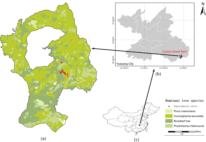
Fig. 1. The location of a) the study area – Loutou forest farm in b) Yueyang of Hunan Province, c) southern China. View larger in new window/tab.
2.2 Data
The used data were obtained from a total of 16 plots in the secondary mixed forests in the Lutou forest farm (Fig. 1a). All the plots were established in 2015 each with the area of 20 m × 20 m. The plots had different topographic features with 8 plots in the areas of sunny slopes and 8 plots in the areas of shady slopes. In the plots, the dominant tree species was C. glauca with mixed tree species including C. eyrei, C. sclerophylla, Cunninghamia lanceolata (Lamb.) Hook., A. fortune and R. latoucheae. Within each of the plots, the values of tree DBH and H were obtained and plot position (X and Y coordinates), elevation, slope, aspect, slope position and canopy density were recorded. Tree DBH and H were measured using a diameter tape and a Blume-Leiss hypsometer, respectively. Plot slope and aspect were measured at four corners of each plot using a compass theodolite and their average values were used as the plot slope and aspect. Plot elevation and slope position were measured using a global positioning system. The information of the plots and trees was shown in Table 1. The statistics of tree variables were given based on different slopes and aspects in Table 2. There were a total of 426 C. glauca trees. Considering the slope and aspect, the dataset was randomly split into two parts: 80% (341 trees) for modeling and 20% (85 trees) for validation. The modeling and validation datasets were further divided into sub-datasets of sunny gentle, sunny steep, shady gentle and shady steep with the number of sample trees varying from 77 to 111 for the modeling dataset, and from 17 to 28 for the validation dataset. The sample means of tree height and DBH measurements among the whole, modeling and validation datasets did not statistically significantly differ from each other at the significant level of 0.05 for all the sub-datasets. Thus, the random divisions were acceptable.
| Table 1. The information of the measured variables for the 16 sample plots (Note: DBH: diameter at breat height; H: tree height; Cg: Cyclobalanopsis glauca; Rs: Rhododendron simsii; Cs: Castanopsis sclerophylla; Ce: Castanopsis eyriei; Lc: Loropetalum chinense; Cl: Cunninghamia lanceolate; Af: Alniphyllum fortune; Ca: Canarium album; Mr: Myrica rubra; Ss: Symplocos sumuntia). | |||||||||
| Sample plot number | Altitude (m) | Slope (degree) | Slope aspect | Slope position | Crown density | Tree composition | Number of trees | Mean DBH (cm) | Mean H (m) |
| 1 | 324 | 19 | sunny | medium | 0.9 | 4Cg 3Rs 1Cs 1Ce 1Lc | 63 | 15.4 | 11.1 |
| 2 | 340 | 17 | sunny | medium | 0.7 | 4Cg 3Rs 2Lc 1Cl | 54 | 12.9 | 9.5 |
| 3 | 312 | 22 | sunny | below | 0.8 | 4Cg 3Rs 2Cl 1Ce | 41 | 14.6 | 10.0 |
| 4 | 310 | 34 | shady | medium | 0.8 | 4Cg 4Rs 1Lc 1Ca | 54 | 12.5 | 9.3 |
| 5 | 330 | 20 | sunny | below | 0.7 | 3Cg 2Ce 2Cl 2Rs 1Mr | 30 | 14.9 | 9.7 |
| 6 | 312 | 32 | sunny | below | 0.8 | 4Cg 3Rs 2Ce 1Lc | 51 | 12.1 | 9.1 |
| 7 | 315 | 33 | sunny | below | 0.7 | 3Cg 3Af 3Rs 1Cl | 53 | 13.1 | 9.0 |
| 8 | 320 | 35 | shady | medium | 0.8 | 4Cg 3Cs 3Lc | 46 | 15.1 | 8.8 |
| 9 | 314 | 35 | shady | medium | 0.7 | 4Cg 2Cs 2Rs 1Af 1Lc | 29 | 14.3 | 11.3 |
| 10 | 318 | 32 | shady | upper | 0.7 | 5Cg 3Rs 2Af | 45 | 13.2 | 9.9 |
| 11 | 302 | 15 | shady | medium | 0.7 | 4Cg 2Af 2Cl 2Lc | 48 | 12.8 | 9.6 |
| 12 | 305 | 20 | shady | medium | 0.7 | 5Cg 2Rs 2Af 1Cl | 81 | 12.7 | 9.5 |
| 13 | 310 | 16 | shady | upper | 0.6 | 5Cg 2Rs 2Cs 1Lc | 50 | 12.3 | 12.5 |
| 14 | 325 | 27 | sunny | medium | 0.8 | 6Cg 2Cs 1Rs 1Cl | 52 | 14.6 | 9.5 |
| 15 | 308 | 30 | sunny | medium | 0.6 | 3Cg 3Cs 2Rs 1Ce 1Af | 40 | 9.5 | 9.6 |
| 16 | 285 | 20 | shady | below | 0.8 | 4Cg 3Cl 1Ce 1Af 1Rs | 100 | 12.1 | 10.3 |
| Table 2. Characteristics of Cyclobalanopsis glauca tree height and diameter at breast height (DBH) measurements for the total, modeling and validation datasets based on sunny-gentle, sunny-steep, shady-gentle and shady-steep (Max: maximum; Min: minimum; SD: standard deviation). | ||||||||||
| Subsets | Sample type | Number | Height (m) | DBH (cm) | ||||||
| Mean | Max | Min | SD | Mean | Max | Min | SD | |||
| Sunny-gentle | Total | 96 | 11.5 | 17.3 | 5.6 | 2.9 | 14.6 | 42.5 | 5.2 | 6.9 |
| Modeling | 77 | 11.5 | 17.3 | 5.6 | 3.0 | 14.7 | 42.5 | 5.2 | 7.3 | |
| Validation | 19 | 11.6 | 16.3 | 6.1 | 2.8 | 14.3 | 22.7 | 7.3 | 5.1 | |
| Sunny-s teep | Total | 86 | 10.3 | 15.4 | 6.5 | 2.2 | 12.9 | 26.0 | 5.0 | 5.1 |
| Modeling | 69 | 10.2 | 15.4 | 6.5 | 2.3 | 13.0 | 26.0 | 5.0 | 5.4 | |
| Validation | 17 | 10.5 | 14.4 | 7.8 | 1.8 | 12.4 | 18.6 | 6.1 | 4.1 | |
| Shady-gentle | Total | 139 | 10.4 | 14.9 | 3.5 | 2.5 | 12.8 | 29.0 | 5.1 | 4.9 |
| Modeling | 111 | 10.4 | 14.8 | 3.5 | 2.5 | 12.9 | 27.2 | 5.1 | 4.9 | |
| Validation | 28 | 10.4 | 14.9 | 5.8 | 2.5 | 12.0 | 29.0 | 5.8 | 4.7 | |
| Shady- steep | Total | 105 | 10.6 | 15.0 | 6.4 | 2.0 | 15.2 | 41.6 | 5.1 | 7.0 |
| Modeling | 84 | 10.7 | 14.7 | 6.4 | 1.9 | 14.8 | 33.4 | 5.1 | 6.3 | |
| Validation | 21 | 10.2 | 15.0 | 6.7 | 2.4 | 16.4 | 41.6 | 5.1 | 9.4 | |
2.3 Modelling of H-DBH relationship and selection of models
A large number of models have been developed to model the relationship of tree H with DBH for different tree species and different regions of same tree species. In this study, a total of 11 commonly used tree H-DBH equations including linear, logarithm linear, exponential, Hyperbolic, Quadratic model and those proposed by Gompertz (1825), Yoshida (1928), Schumacher (1939), Richards (1959), Näslund (1937) and Wykoff et al. (1982), were selected to fit the tree H-DBH relationship of C. glauca secondary forests (Table 3). Because the H-DBH relationship may be different depending on topographic features and also affected by the competition among trees, modeling the H-DBH relationship was conducted under the different slopes and aspects including sunny-steep, sunny-gentle, shady-steep and shady-gentle and also by introducing a tree competition variable into the models in this study. The differences in the growth of H and DBH due to different slopes and aspects and the corresponding growth process were analyzed using Chow’s F-test based on the sums of square residuals of H predictions. If the growth between the sunny and shady slope was different significantly, the differences of the growth process among sunny-gentle, sunny-steep, shady-gentle and shady-steep slope were further tested. A statistical test result of no significant difference implied that the tree H-DBH relationship of C. glauca trees was basically consistent under different slopes and aspects.
| Table 3. The basic models used for comparison of modeling the relationship of tree height (H) with diameter at breast height (DBH) (Note: D is DBH; a, b, c and d are model parameters; M#: model numbers). | |||||
| M# | Model | References | M# | Model | References |
| M1 | Linear | M7 | Yoshida (1928) | ||
| M2 | Log | M8 | Schumacher (1939) | ||
| M3 | Exponential | M9 | Richards (1959) | ||
| M4 | Hyperbolic curve | M10 | Huang and Titus (1992) | ||
| M5 | Quadratic | M11 | Wykoff et al. (1982) | ||
| M6 | Gompertz (1825) | ||||
2.4 The improved Hegyi competition index
As a famous and simple index, Hegyi CI has been widely used for quantifying competition degree among trees in forest stands (Vanclay et al. 2013; Timilsina and Staudhammer 2013). Hegyi CI is defined based on the DBH values of a target tree and its competitors and the horizontal distances of the competitors to the target tree and easy to obtain because the values of tree H are not taken into account. That is, Hegyi CI ignores the impact of tree H from the competitors. However, in a forest, because trees grow with biomass accumulated by absorbing light, water and nutrients, a 3-dimensional space is needed, in which trees compete with each other for gaining the resources. Thus, Hegyi CI should be improved by defining it in a 3-dimensional space. Considering the values of tree H are often difficult to gain, in this study the relative relationships of tree H between competitors and a target tree were taken into account. The widely used methods of selecting competitors include the uses of crown overlap, nearest neighbors and Thiessen polygon. Moreover, previous studies show that four trees closest to the target tree often have obvious effects on the growth of the target tree because the four nearest neighbors are most likely competing with the target tree for the resources needed for growing (Hui et al. 2018). In addition, this method is simplest. Therefore, four nearest trees from the target tree were regarded as competition trees in this study. The original Hegyi CI is calculated as follows:

where i is the target tree, j represents the competing tree j, Di is the DBH of the target tree, Dj is the DBH of the competing tree j, Lij is the distance between the target tree i and competing tree j, and N is the number of the competing trees. Considering the impact of tree H from the competitors, given a distance and DBH a competition tree taller than the target tree should have a greater impact on the growing of the target tree than the one shorter than the target tree. This is mainly because the former occupies more space vertically and may have a strong root system than the latter. Moreover, the former often shades the target tree. Thus, the improved Hegyi CI focused on the adjustment of competition effect by changing the contributions of the diameters of the competing trees. The adjusted diameter of the competitor j was calculated as follows:
![]()
where k is a generalized parameter and functions to reflect the contribution from the height Hj of the competing tree j by modifying its value of DBH. When the target tree is taller than a competing tree (that is, Hi > Hj), the impact of the competing tree on the growth of the target tree is assumed to be weaker and thus k could be smaller than 1. When the target tree is equal to and shorter than a competing tree (that is, Hi ≤ Hj), the impact of the competing tree on the growth of the target tree is assumed to be stronger and thus k could be equal to or larger than 1. Theoretically, the k could be any value and determined by the ratio of the height of a competing tree to the height of the target tree. For simplification, in this study we only tested two values, that is, k = 0.5 for Hi > Hj, and k = 1 for Hi ≤ Hj.
The improved Hegyi CI is accounted for by Eq. 1 and Eq. 2 together and denoted with Hegyi_I. When the height of the target tree is higher than that of the competition tree, the effect of the Hj on the target tree is indirectly accounted for by reducing the contribution from its DBH to ![]() , that is, weakening the impact of the competitor. When the target tree is shorter than the competing tree, the contribution from the DBH of the competing tree is not adjusted, which means that the impact of the taller competitor is relatively enhanced compared with that of the shorter competitor. Moreover, the improvement does not lead to the need to accurately measure the heights of trees. Instead, the relative relationships between the height of the target tree and the heights of the competing trees can be easily and visually determined.
, that is, weakening the impact of the competitor. When the target tree is shorter than the competing tree, the contribution from the DBH of the competing tree is not adjusted, which means that the impact of the taller competitor is relatively enhanced compared with that of the shorter competitor. Moreover, the improvement does not lead to the need to accurately measure the heights of trees. Instead, the relative relationships between the height of the target tree and the heights of the competing trees can be easily and visually determined.
The original Hegyi CI is defined in a 2-dimensional space. The improved Hegyi CI indirectly takes into account the effect of tree H from competitors and quantifies the impacts of four nearest competing trees on the target tree from both horizontal and vertical directions. In this study, the effects of these two CIs on the H-DBH relationship were compared by analyzing their correlations with tree H and DBH and assessing the prediction accuracies of tree H using the H-DBH models in which the original and improved, Hegyi and Hegyi_I, were added as a predictor, respectively.
2.5 Model assessment
In this study, the whole modeling dataset was first used to develop the models and make the predictions of tree H. The modeling dataset was then divided into sunny and shady slope sub-datasets and the two sub-datasets were respectively utilized to build the models and predict the tree H. The residuals of the tree H predictions from the models using the whole modeling dataset and two sub-datasets respectively were calculated and Chow’s F-tests were conducted to examine if the corresponding parameters of the same models obtained using the sunny and shady slope sub-datasets were statistically significantly different from that of the whole dataset (Chow, 1960). The tests were carried out based on the sums of the squared residuals. The Chow’s F-test equation was:

where given a model, let SSRT, SSR1 and SSR2 be the sums of squared residuals from the H-DBH models using the whole modeling dataset and the sunny and shady slope sub-datasets, respectively. SSR4 = SSR1 + SSR2, SSR5 = SSRT – SSR4, n1 and n2 are the numbers of the observations for the sunny and shady slope sub-datasets and m is the number of the arguments. In Chow’s F-test, the hypothesis is given as follows: given a model, aspect does not affect the H-DBH relationship. If the whole modeling dataset is divided into two sub-datasets corresponding to the sunny and shady slope and these two sub-datasets are fit using the same model, the sums of the squared residuals from two models that have the same structure should have the same normal distribution. If the model structures are the same, the total sum of the squared residuals from two sub-datasets, S1 + S2, should not statistically significantly different from that, SR, obtained using the whole modeling dataset. Therefore, the coefficients of the models, that is, the model structures, are statistically the same. If F statistics is greater than the critical value of F at the significance level of 0.05, the hypothesis is rejected, implying that the division of the sunny and shady slope sub-datasets led to significant difference of sums of the square residuals, that is, different coefficients of the models. If so, the further divisions of the sunny slope into sunny-steep and sunny-gentle and the shady slope into shady-steep and shady-gentle, and the corresponding Chow’s F-tests were conducted.
Moreover, a total of eleven basic models were compared to fit the H-DBH relationship of C. glauca trees (Table 3). The H-DBH models were evaluated using the coefficient of determination (R2) and root mean square error (RMSE) between the observed and predicted values of tree H, and Akaike information criterion (AIC). Through the assessment results, the optimal model was selected. Finally, the original Hegyi and the improved Hegyi_I were respectively introduced into the selected models as a predictor and the resulting models were used to predict tree H. For the same model, the prediction results from the model without CI and the models with Hegyi and Hegyi_I were compared to verify whether or not the introduction of Hegyi and Hegyi_I significantly improved the predictions of tree H.
3 Results
3.1 The effects of slope and aspect on the H-DBH relationship
In Table 4, the H-DBH relationship of Cyclobalanopsis glauca trees was fit using the eleven models (M1 to M11) and the whole modeling dataset. The relationship was further fit using the sub-datasets of sunny-slope, shady-slope, steep-slope and gentle-slope and the optimal model was selected for each of the sub-datasets in Table 5. The results of Chow’s F-test showed that the division of the modeling dataset into sunny and shady slopes, and steep and gentle slopes led to the different structures of the H-DBH relationship because there were statistically significant differences of the sums of square residuals from the H predictions of all the models at the significant level of 0.05. Similarly, when the modeling dataset was divided into sunny-steep, sunny-gentle, shady-steep and shady-gentle slope, Chow’s F-test also indicated that the sums of square residuals from the H predictions of all the models significantly differed from each other, implying the significantly different H-DBH relationship structures for almost all the models obtained by the sub-datasets.
| Table 4. The results of eleven basic models (M1 to M11) used for fitting the H-DBH relationship using the whole modeling dataset (H is tree height; DBH is diameter at breast height; a, b, c and d are model parameters; RMSE and R2 respectively are root mean square error and coefficient of determination between the observed and estimated values of H; and SSR is the sum of squared residuals). | |||||||
| Model parameter | Model evaluation | ||||||
| M# | a | b | c | d | R2 | SSR | RMSE |
| M1 | 0.321 | 6.241 | 0.624 | 972.654 | 1.511 | ||
| M2 | 4.735 | –1.323 | 0.683 | 821.522 | 1.389 | ||
| M3 | 3.529 | 0.043 | 0.670 | 854.983 | 1.417 | ||
| M4 | 19.897 | 216.848 | 10.988 | 0.685 | 816.203 | 1.384 | |
| M5 | –0.0097 | 0.6517 | 3.8716 | 0.679 | 831.126 | 1.397 | |
| M6 | 15.02 | 1.471 | 0.116 | 0.686 | 813.143 | 1.382 | |
| M7 | 10.672 | 156.574 | 2.024 | 5.169 | 0.686 | 811.589 | 1.380 |
| M8 | 16.936 | 5.552 | 0.676 | 839.931 | 1.404 | ||
| M9 | 15.949 | 0.764 | 0.071 | 0.685 | 814.723 | 1.383 | |
| M10 | 0.874 | 0.235 | 0.682 | 821.891 | 1.389 | ||
| M11 | 2.87 | –6.62 | 0.681 | 826.471 | 1.393 | ||
| Table 5. The results of the optimal models selected from the eleven basic models (M1 to M11) used for fitting the H-DBH relationship for each of the sub-datasets including sunny, shady, steep and gentle slope, and sunny-steep, sunny-gentle, shady-steep and shady-steep (a, b and c are model parameters; RMSE and R2 respectively are root mean square error and coefficient of determination between the observed and estimated values of H; SSR is the sum of squared residuals; and AIC is Akaike information criterion). | ||||||||
| Dataset | Model # | Model parameter | Model evaluation | |||||
| a | b | c | R2 | SSR | RMSE | AIC | ||
| Sunny slope | M6 | 16.704 | 1.416 | 0.094 | 0.695 | 394.29 | 1.472 | 146.7 |
| Shady slope | M6 | 13.945 | 1.597 | 0.140 | 0.702 | 379.41 | 1.247 | 113.7 |
| Steep slope | M2 | 3.922 | 0.451 | 0.714 | 232.83 | 1.104 | 85.4 | |
| Gentle slope | M6 | 15.816 | 1.757 | 0.124 | 0.720 | 492.06 | 1.447 | 130.3 |
| Sunny-steep | M2 | 4.253 | –0.249 | 0.622 | 154.55 | 1.341 | 54.4 | |
| Sunny-gentle | M6 | 16.817 | 1.591 | 0.109 | 0.754 | 200.08 | 1.444 | 76.5 |
| Shady-steep | M3 | 4.094 | 0.359 | 0.818 | 73.03 | 0.834 | –34.1 | |
| Shady-gentle | M6 | 14.119 | 2.184 | 0.169 | 0.706 | 255.58 | 1.356 | 92.7 |
3.2 Selection of optimal H-DBH models
In Table 4, when the whole modeling dataset was used, the values of R2 and RMSE obtained using all the models statistically were not significantly different from each other at the significant level of 0.05 except for M1 led to poorer performance. With the division of the sunny, shady, steep and gentle slope sub-datasets, the optimal model M6 was obtained based on the smallest RMSE and AIC and the largest R2 for all the sub-datasets except for the steep slope in which the model M2 performed best (Table 5). With the division of the sunny-steep, sunny-gentle, shady-steep and shady-gentle slope plots, overall the values of R2 or RMSE were similar among the non-linear models (M2 to M11), while the linear model M1 led to smaller R2 and larger RMSE (Table 5). Based on the smallest AIC, however, M2 was selected for the sunny-steep and M6 was selected for the sunny-gentle and shady-gentle, while M3 was chosen for the shady-steep (Table 5).
3.3 Effect of competition index
The correlation coefficients of the original Hegyi and the improved Hegyi_I with tree H and DBH showed similar trends (The coefficents omitted due to the limited space). The improved Hegyi_I had the absolute coefficients varying from 0.37 to 0.65 with H and from 0.37 to 0.67 with DBH for the whole modeling dataset and all the sub-datasets. The corresponding values of the original Hegyi ranged from 0.25 to 0.53 with H and from 0.26 to 0.55 with DBH. This implied that the improved Hegyi_I increased the correlation and enhanced the effect of tree H from the competitors.
The Hegyi_I and Hegyi as an independent variable were respectively added into each parameter of the same H-DBH model selected for each of the sunny-steep, sunny-gentle, shady-steep and shady-gentle sub-datasets. The fittings led to different structures of the models and the optimal model structure was then selected based on the largest R2 and smallest RMSE. In Table 6, compared with those without CI, overall, adding the original Hegyi into the models increased the R2 values and reduced the RMSE values for all the sub-datasets. The improvements were further enhanced by introducing the improved Hegyi_I into the models (Table 6).
| Table 6. The comparison of the results using the optimal models without and with the original Hegyi and improved Hegyi_I involved for sunny-steep, sunny-gentle, shady-steep and shady-gentle slope forests (a, b, c, f and g are model parameters; STE is the standard error of the estimated parameter; RMSE and R2 respectively are root mean square error and coefficient of determination between the observed and estimated values of H; SSR is the sum of squared residuals; and the symbol * implying the model parameter statistically is significantly different from zero at the significant level of 0.05). | ||||||||
| Model characteristics | Model parameter | Model evaluation | ||||||
| a (STE) | b (STE) | c (STE) | f (STE) | g (STE) | RMSE | SSR | R2 | |
| Sunny-steep slope | ||||||||
| *4.253(0.362) | –0.249(0.908) | 1.341 | 154.550 | 0.622 | ||||
| *10.198(0.906) | –0.921(1.083) | 0.071(0.063) | 1.330 | 152.192 | 0.628 | |||
| *3.693(0.463) | 1.712(1.367) | *–0.182(0.086) | 1.312 | 148.219 | 0.638 | |||
| Sunny-gentle slope | ||||||||
| *16.817(0.924) | *1.591(0.178) | *0.109(0.019) | 1.444 | 200.078 | 0.754 | |||
| *16.858(0.981) | *1.542(0.283) | *0.107(0.022) | 0.006(0.026) | 1.443 | 199.967 | 0.754 | ||
| *17.259(0.967) | *1.119(0.130) | *0.093(0.016) | *0.015(0.004) | 1.348 | 174.524 | 0.786 | ||
| Shady-steep slope | ||||||||
| *4.094(0.195) | *0.359(0.017) | 0.834 | 73.031 | 0.818 | ||||
| *4.415(0.245) | *0.339(0.018) | *–0.022(0.009) | 0.811 | 69.059 | 0.828 | |||
| *4.864(0.279) | *0.316(0.018) | *–0.017(0.004) | 0.759 | 60.472 | 0.849 | |||
| Shady-gentle slope | ||||||||
| *14.119(0.581) | *2.184(0.355) | *0.169(0.026) | 1.356 | 255.579 | 0.706 | |||
| *14.301(0.645) | *1.928(0.402) | *0.162(0.029) | –0.298(0.250) | 1.363 | 258.098 | 0.703 | ||
| *13.906(0.504) | *2.850(0.569) | *0.191(0.027) | *–0.044(0.021) | 1.341 | 249.868 | 0.712 | ||
For the sunny-steep, compared with the optimal model M2 without the CIs, the additions of both the original Hegyi and improved Hegyi_I into M2 increased the prediction accuracy of tree H but the parameter corresponding to the original Hegyi was not significantly different from zero at the significant level of 0.05, while the parameter corresponding to the improved Hegyi_I significantly differed from zero. The similar results were obtained for the sunny-gentle and shady-gentle sub-datasets in which the model M6 was selected. For the shady-steep, the model parameters corresponding to the original Hegyi and the improved Hegyi_I in the model M3 were statistically significantly different from zero. This implied that introducing the improved Hegyi_I into the selected models statistically resulted in significantly different model structures of the H-DBH relationship for all the sub-datasets and increased the prediction accuracy of tree H compared with the models with and without the original Hegyi, while the effect of adding the original Hegyi into the models was significant only for the shady-steep.
In Table 7, significant difference tests of the average absolute residuals of the H predictions from zero using the models without and with the original Hegyi and the improved Hegyi_I were conducted using the student-T distribution. The test results showed that at the significant level of 0.05 the average absolute residuals were not significantly different from zero for all the sub-datasets and all the models without and with the original Hegyi and the improved Hegyi_I. However, the absolute average residuals of the predictions decreased due to the inclusions of the original Hegyi and the improved Hegyi_I in the models. This indicated that compared with the models without the CIs, the models with the original Hegyi increased the prediction accuracy of tree H and the accuracy was further increased by the models with the improved Hegyi_I.
| Table 7. Significant difference test of the average absolute residuals from zero using the models without and with the competition indices Hegyi CI and Hegyi_I CI involved (δ1 is the average of the absolute residuals for the model without competition index, δ2 is the average of the absolute residuals for the model with the original Hegyi and δ3 is the average of the absolute residuals for the model with the improved Hegyi_I). | ||||||||||
| Sub-datasets | Model | δ1 | δ2 | δ3 | δ1 vs. δ2 | δ1 vs. δ3 | δ2 vs. δ3 | |||
| T value | P value | T value | P value | T value | P value | |||||
| Sunny-steep | M2 | 1.10* | 1.05* | 0.98* | 1.635 | 0.106 | 2.310 | 0.023 | 1.578 | 0.118 |
| Sunny-gentle | M6 | 1.18* | 1.12* | 1.09* | 0.405 | 0.686 | 1.748 | 0.084 | 0.303 | 0.763 |
| Shady-steep | M3 | 0.65* | 0.62* | 0.57* | 1.292 | 0.199 | 2.386 | 0.019 | 1.903 | 0.060 |
| Shady-gentle | M6 | 1.11* | 1.09* | 1.05* | 0.676 | 0.500 | 1.906 | 0.059 | 1.495 | 0.137 |
In Table 7, given a sub-dataset the significant difference between any two average absolute residuals of the H predictions from the models without and with the CIs was also examined. When the models without the original Hegyi were compared with the models that contained the original Hegyi, the P-values for all the sub-datasets were greater than 0.1, indicating that adding the original Hegyi into the models did not significantly reduce the average absolute residuals. Compared with the models without the improved Hegyi_I, the models with the improved Hegyi_I led to the P-values of smaller than 0.05 for both the sunny-steep and shady-steep and smaller than 0.1 for the sunny-gentle and shady-gentle. This suggested that at the significant level of 0.1, the models with the improved Hegyi_I significantly increased the prediction accuracy of tree H. Moreover, when the models with the original Hegyi were compared with the models containing the improved Hegyi_I, all the P-values were greater than 0.1 except for the shady-steep sub-dataset that led to the P-value smaller than 0.1 but greater than 0.05.
In Fig. 2, the observations of tree H were graphed against the observations of DBH together with the fit curves for the whole dataset and sub-datasets. When the whole dataset was used, the fit curve obviously led to the overestimations and underestimations for the small and large values of tree H. The divisions of the whole dataset into the sub-datasets reduced the overestimations and underestimations.
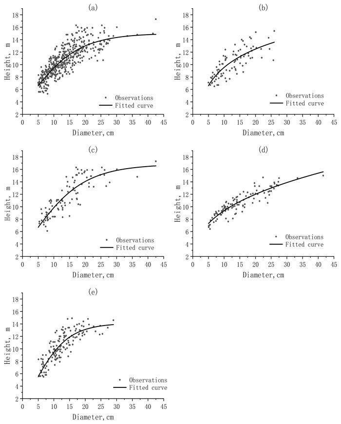
Fig. 2. The scattered distributions and fitted curves of the observed height (H) against the observed diameter (DBH) for a) the whole dataset and different sub-datasets: b) sunny-steep; c) sunny-gentle; d) shady-steep; and e) shady-gentle.
In Table 8, the RMSE values of the predicted H from the whole model and the separate models without and with the CIs were compared based on the validation dataset. Compared to the whole model, the separate models from the sunny-steep, sunny-gentle, shady-steep and shady-gentle slope reduced the RMSE values by 1.83% to 21.62% depending on the sub-datasets. All the decreases were significantly different from zero except for the model for the sunny-steep sub-dataset. This implied that the H-DBH relationship varied with the slopes and aspects and showed different structures. Thus, separately developing the H-DBH relationship at different slopes and aspects significantly improved the predictions of tree H. Moreover, compared with the whole model, all the separate models with the original Hegyi and the improved Hegyi_I, respectively, led to the significant reduction of RMSE for the predictions of tree H (Table 8). In addition, compared with the separate models that contained the original Hegyi, the separate models with the improved Hegyi_I further reduced the values of RMSE for the predictions of tree H but the significant decreases happened only for the sunny-gentle and shady-steep sub-datasets.
| Table 8. The improvement of tree H predictions using separate models at different slopes and aspects by comparison with the whole model based on root mean square error (RMSE) between the predicted and observed values of the validation dataset (W is the whole model, S1 is the separate models without competition index, S2 is the separate models with the original Hegyi and S3 is the separate models with the improved Hegyi_I. | ||||||||
| Datasets | RMSE | Percentage of reduced error (%) | ||||||
| W | S1 | S2 | S3 | W vs. S1 | W vs. S2 | W vs. S3 | S2 vs. S3 | |
| Sunny-steep slope | 1.366 | 1.341 | 1.33 | 1.312 | 1.83 | 2.64 | 3.95 | 1.35 |
| Sunny-gentle slope | 1.635 | 1.444 | 1.443 | 1.348 | 11.68 | 11.74 | 17.55 | 6.58 |
| Shady-steep slope | 1.064 | 0.834 | 0.811 | 0.759 | 21.62 | 23.78 | 28.66 | 6.41 |
| Shady-gentle slope | 1.412 | 1.356 | 1.363 | 1.341 | 3.97 | 3.47 | 5.03 | 1.61 |
4 Discussion
There are many factors and variables affecting the growth of tree H and DBH and thus the H-DBH relationship, such as elevation (Scaranello et al. 2011), soil (Gauthier et al. 2018), slope and aspect (Rohner et al. 2013), etc. Slope and aspect cause the differences of light trees need for growing and thus are the most important variables that have effects on the H-DBH relationship of trees and forest productivity (Kravkaz et al. 2018). Light intensity and time of illumination on sunny slopes and shady slopes are quite different, which leads to different survival rates and growth rates of trees on sunny slopes and shady slopes (Motsinger et al. 2010). On the other hand, steep slope areas often have poorer soil nutrients and less water supply than gentle slope areas and the different amounts of resources trees need for growing would affect the H-DBH relationship of trees (Scharnweber et al. 2011). Rohner et al. (2013) found that oak trees grow faster in diameter at lower elevation and gentler slope areas than at higher elevation and steeper slope areas. The results of Chow’s F-test based on the sums of square residuals in this study showed that the slope and aspect had significant effects on the H-DBH relationship of C. glauca trees and the H-DBH relationship should be modelled by considering different slopes and aspects, which supported the conclusion of previous studies for other tree species. Thus, the H-DBH relationship should be modeled based on sunny-steep, sunny-gentle, shady-steep and shady-gentle slope forests.
Various nonlinear equations with high accuracy and strong ability of predicting H have been widely used to model the H-DBH relationship of different tree species at different conditions (Ozcelik et al. 2014; Sancheza et al. 2003). However, because the H-DBH relationship varies depending on different tree species and different site conditions, the selection of nonlinear equations is necessary and critical to optimize modeling the H-DBH relationship for C. glauca trees at different site conditions including the sunny-steep, sunny-gentle, shady-steep and shady-gentle slopes. In this study, it was found that the linear model had significantly poorer performance than the nonlinear equations. When the whole modeling dataset was used, the nonlinear equations resulted in only slight differences of accuracy for predicting H of the trees based on RMSE and R2. However, the log transformation equation (M2) and exponential equation (M3) were optimal to model the H-DBH relationship for the sunny- and shady-steep slope forests, while the Gompertz’s equation (M6) had best performance to explain the H-DBH relationship for the sunny- and shady-gentle slope forests. This implied that the H-DBH relationship had different structures due to different site conditions caused by the aspects and slopes.
Tree competition for obtaining resources (light, water and nutrients) is a complicated process and various CIs have been developed to quantify the degree of tree competition (Burkhart and Tome 2012). However, the performance of CIs is often site-specific and varies depending on forest types and site conditions (Contreras et al. 2011). Because of being defined in a 2-dimensional geographic space, distance-dependent CIs are usually superior compared with distance-independent CIs (Burkhart and Tome 2012). However, trees grow and compete for obtaining the resources in a 3-dimensional space, the distance-dependent CIs often ignore the impact of tree H from competitors mainly due to the difficulty for measuring tree H (Burkhart and Tome 2012).
Because of its simplification and effectiveness, Hegyi CI has been most commonly utilized to quantify the competitive impact (Saha et al. 2014; Vanclay et al. 2013; Timilsina and Staudhammer 2013). However, Hegyi is defined based on tree DBH values and distances among trees in a 2-dimensional geographic space and ignores the impacts of H from competitors on a target tree. In this study, an improved Hegyi_I was developed by taking into account into the original Hegyi the relative relationships of H for competitors to the target tree and representing the impacts of tree H from the competitors through adjusting the contributions of DBH to the CI when the heights of competitors were different from the target tree H. Thus, the improved Hegyi_I was indirectly defined in a 3-dimensional space to quantify the competition degree. The correlation analysis showed that the improved Hegyi_I, to some extent, reflected the effects of tree H from competitors in addition to their DBH values and distances to the target tree and was more appropriately used as a CI than the original Hegyi. Moreover, although, compared with the models without the original Hegyi and improved Hegyi_I, the inclusions of both CIs in the H-DBH models increased the prediction accuracy of tree H for all the sub-datasets, the accuracy increases by the improved Hegyi_I were statistically significant at the significant level of 0.1 but not by the original Hegyi. The improved Hegyi_I is generalized in which, theoretically, the k quantifies the contribution of height from each competing tree to the improved competing index and should be determined using the ratio of the height from the competing tree to the height of the target tree. However, this requires the measurements of tree heights and makes the improved index hardly applicable. For simplification, in this study only k = 0.5 for Hi > Hj and k = 1 for Hi ≤ Hj were examined and the obtained results showed promising. The simplification would not weaken the generalization of the improved Hegyi_I. In the future study, optimal k values should be explored.
The objective of developing the improved Hegyi_I is to improve the estimation of tree H. That means that the heights of the target tree and its competitors are unknown. However, the calculation of the improved Hegyi_I still requires the information of the relative relationship of the target tree H to the H values of its competitors. The information of the relative relationship does not need accurate measurements of the tree heights and can be obtained by approximate or visual estimation. However, currently there have been rare cases in which relative heights of four nearest trees for each target tree in a plot were obtained or the heights of the trees were visually estimated. Tree heights are often measured with a hypsometer instead of visual observations, which could give an overly positive view of the accuracy. The proposed index could still be used, especially in forests where visual estimation of height is feasible. In the future, the approximate values of tree heights can be yielded using high spatial resolution stereo images by photogrammetric measurements or using airborne or terrestrial laser scanning LiDAR data. Thus, the improved Hegyi is promising for its application.
In addition, the mixed-effect models have been commonly applied in practice for their advantages in the application of repeated and multi-level data and accounting for random effects. This is especially true for mixed forests. In this study, the mixed-effect models were not used mainly because the site conditions of the plots in the study area were similar except for slope and aspect. Thus, we would like to focus on the influence of slope and aspect on the H-DBH relationship. Moreover, the mixed-effect models are relatively complex and computation-intensive, while the influence of slope and aspect on the H-DBH relationship could be clarified by using simple regression models to be easily and separately developed based on different categories including sunny-steep, sunny-gentle, shady-steep and shady-gentle. Therefore, our research objectives could be easily achieved by using the relatively simpler and applicable method. In the future study, the mixed-effect models should be explored.
Finally, considering the slope and aspect, the dataset was randomly split into modeling and validation datasets. How the random division influences the results of the analysis is not clear. This can be achieved by repeatedly conducting the random divisions and corresponding modeling and analyses with a reliable number of runs such as greater than 30 times. But, this will lead to a huge amount of work. Due to the limited time and space, we did not carry out the analyses in this study. In the future study, the simulations can be done.
5 Conclusions
In this study, in order to improve the predictions of Cyclobalanopsis glauca tree H, the effects of slope and aspect on the H-DBH relationship were investigated using Chow’s F-test based on the sums of square residuals and assessment of H predictions from models. A total of eleven equations were compared and selected to optimize modeling the H-DBH relationship. Moreover, an improved Hegyi_I was developed and the effects of both the original Hegyi and the improved Hegyi_I on the H-DBH relationship were analyzed by separately introducing them into the selected models. The results showed that 1) The effects of slope and aspect on the H-DBH relationship of C. glauca trees were significant at the significant level of 0.05; 2) The H-DBH relationship varied depending on different slopes and aspects, which led to different optimal models, including the log transformation model (M2) and exponential model (M3) for the sunny- and shady-steep slope forests and the Gompertz’s model (M6) for both the sunny- and shady-gentle slope forests. Compared with the model from the whole dataset, the division of the dataset into the sub-datasets of the sunny-steep, sunny-gentle, shady-steep and shady-gentle slope significantly reduced the RMSE values; 3) Compared with the selected models without the CIs, adding the original Hegyi and the improved Hegyi_I into the H-DBH models increased the prediction accuracy of tree H for all the sub-datasets but the significant improvements were achieved only by the models that contained the improved Hegyi_I at the significant level of 0.1. This indicated that the improved Hegyi_I, to some extent, more accurately quantified the competition degree of trees in the C. glauca mixed forests than the original Hegyi. This study implied that modeling the H-DBH relationship under different slopes and aspects, coupled with the inclusion of the improved Hegyi_I, provided the great potential to improve the prediction accuracy of tree H in the C. glauca mixed forests.
Acknowledgements
This study was financially supported by the forestry public industry scientific research project (No: 201504301).
References
Alder D. (1979). A distance-independent tree model for exotic conifer plantations in East Africa. Forest Science 25(1): 59–71.
Amaro A., Reed D., Tome M., Themido I. (1998). Modelling dominant height growth: eucalyptus plantations in Portugal. Forest Science 44(44): 37–46.
Bella I.E. (1971). A new competition model for individual tree. Forest Science 17: 367–372.
Biging G.S., Dobbertin M. (1995). Evaluation of CIs in individual tree growth-models. Forest Science 41: 360–377.
Brand D.G., Magnussen S. (1988). Asymmetric, two-sided competition in even-aged monocultures of red pine. Canadian Journal of Forest Research 18(7): 901–910. https://doi.org/10.1139/x88-137.
Burkhart H.E., Tome M. (2012). Indices of individual-tree competition. In: Modeling forest trees and stands. Springer, Dordrecht. p. 201–232. https://doi.org/10.1007/978-90-481-3170-9_9.
Calama R., Montero G. (2004). Interregional nonlinear height–diameter model with random coefficients for stone pine in Spain. Canadian Journal of Forest Research 34(1): 150–163. https://doi.org/10.1139/x03-199.
Canham C.D., LePage P.T., Coates K.D. (2004). A neighborhood analysis of canopy tree competition: effects of shading versus crowding. Canadian Journal of Forest Research 34(4): 778–787. https://doi.org/10.1139/x03-232.
Chow G.C. (1960). Tests of equality between sets of coefficients in two linear regressions. Econometrica 28(3): 591–605. https://doi.org/10.2307/1910133.
Contreras M.A., Affleck D., Chung W. (2011). Evaluating tree competition indices as predictors of basal area increment in western Montana forests. Forest Ecology and Management 262(11): 1939–1949. https://doi.org/10.1016/j.foreco.2011.08.031.
Daniels R.F. (1976). Simple competition indices and their correlation with annual loblolly-pine tree growth. Forest Science 22: 454–456.
Daniels R.F., Burkhart H.E., Clason T.R. (1986). A comparison of competition measures for predicting growth of loblolly pine trees. Canadian Journal of Forest Research 16(6): 1230–1237. https://doi.org/10.1139/x86-218.
de Mendonca A.R, Calegario N, da Silva G.F. (2011). Height diameter relationship and growth in height the dominant and codominant trees model to Pinus caribaea var. hondurensis. Scientia Forestalis 39(90): 151–160.
Ercanli I. (2015). Nonlinear mixed effect models for predicting relationships between total height and diameter of oriental beech trees in Kestel, Turkey. Revista Chapingo Serie Ciencias Forestales Y Del Ambiente 21(2): 185–202. https://doi.org/10.5154/r.rchscfa.2015.02.006.
Fast A.J., Ducey M.J. (2011). Height-diameter equations for select New Hampshire tree species. Northern Journal of Applied Forestry 28(3): 157–160. https://doi.org/10.1093/njaf/28.3.157.
Fekedulengn D., Siurtain M.P.M., Colbert J.J. (1999). Parameter estimation of nonlinear growth models in forestry. Silva Fennica 33(4): 327–336. https://doi.org/10.14214/sf.653.
Gauthier M.M., Jacobs D.F. (2018). Ecophysiological drivers of hardwood plantation diameter growth under non-limiting light conditions. Forest Ecology and Management 419–420: 220–226. https://doi.org/10.1016/j.foreco.2018.03.036.
Gompertz B. (1825). On function expressive human mortality, new method life contingencies. Philosophical Transactions of the Royal Society of London 115: 513–583. https://doi.org/10.1098/rstl.1825.0026.
Hegyi F. (1974). A simulation model for managing Jackpine stands. In: Fries J. (ed.). Growth models for tree and stand simulation. Royal College of Forestry. p. 74–90.
Huang S., Titus S.J., Wiens D.P. (1992). Comparison of nonlinear height–diameter functions for major Alberta tree species. Canadian Journal of Forest Research 22(9): 1297–1304. https://doi.org/10.1139/x92-172.
Hui G.Y., Wang Y., Zhang G.Q., Zhao Z.G., Bai C., Liu W.Z. (2018). A novel approach for assessing the neighborhood competition in two different aged forests. Forest Ecology and Management 422: 49–58. https://doi.org/10.1016/j.foreco.2018.03.045.
Kalbi S., Fallah A., Bettinger P., Shataee S., Yousefpour R. (2018). Mixed-effects modeling for tree height prediction models of Oriental beech in the Hyrcanian forest. Journal of Forestry Research 29(5): 1195–1204. https://doi.org/10.1007/s11676-017-0551-z.
Kearsley E., Moonen P.C.J., Hufkens K., Doetterl S., Lisingo J., Bosela F.B., Boeckx P., Beeckman H., Verbeeck H. (2017). Model performance of tree height-diameter relationships in the central Congo Basin. Annals of Forest Science 74(1): 7. https://doi.org/10.1007/s13595-016-0611-0.
Lappi J. (1997). A longitudinal analysis of height/diameter curves. Forest Science 43: 555–570.
Larjavaara M., Muller-Landau H.C. (2013). Measuring tree height: a quantitative comparison of two common field methods in a moist tropical forest. Methods of Ecology and Evolution 4(9): 793–801. https://doi.org/10.1111/2041-210X.12071.
Larsen D.R., Hann D.W. (1987). Height–diameter equations for seventeen tree species in southwest Oregon. Oregon State University, Forest Research Laboratory, Corvallis, Research Paper 49.
Kravkaz-Kuscu I.S., Sariyildiz T., Cetin M., Yigit N., Sevik H., Savaci G. (2018). Evaluation of the soil properties and primary forest tree species in Taskopru (Kastamonu) district. Fresenius Environmental Bulletin 27(3): 1613–1617. https://doi.org/10.15244/pjoes/78475.
Krumland B.E., Wensel L.C. (1978). A generalized height–diameter equation for coastal California species. Western Journal of Applied Forestry 3(4): 113–115. https://doi.org/10.1093/wjaf/3.4.113.
Ledermann T. (2010). Evaluating the performance of semi-distance-independent competition indices in predicting the basal area growth of individual trees. Canadian Journal of Forest Research 40(4): 796–805. https://doi.org/10.1139/X10-026.
Li F.R., Lu J., Chen D.S. (2008). Individual-based competition analysis for secondary forest in northeast China. Journal of Korean Forest Society 97(5): 501–507.
Lorimer C.G. (1983). Tests of age-independent competition indices for individual trees in natural hardwood stands. Forest Ecology and Management 6(4): 343–360. https://doi.org/10.1016/0378-1127(83)90042-7.
MacPhee C., Kershaw J.A., Weiskittel A.R., Golding J., Lavigne M.B. (2018). Comparison of approaches for estimating individual tree height-diameter relationships in the Acadian forest region. Forestry 91(1): 132–146. https://doi.org/10.1093/forestry/cpx039.
Martin G.L., Ek A.R. (1984). A comparison of competition measures and growth models for predicting plantation red pine diameter and height growth. Forest Resources 30(3): 731–743.
Mensah S., Pienaar O.L., Kunneke A., du Toit B., Seydack A., Uhl E., Pretzsch H., Seifert T. (2018). Height-diameter allometry in South Africa’s indigenous high forests: Assessing generic models performance and function forms. Forest Ecology and Management 410: 1–11. https://doi.org/10.1016/j.foreco.2017.12.030.
Motsinger J.R., Kabrick J.M., Dey D.C., Henderson D.E., Zenner E.K. (2010). Effect of midstory and understory removal on the establishment and development of natural and artificial pin oak advance reproduction in bottomland forests. New Forests 39(2): 195–213. https://doi.org/10.1007/s11056-009-9164-5.
Opie J.E. (1968). Predictability of individual tree growth using various definitions of competing basal area. Forest Science 14: 314–323.
Parresol B.R. (1992). Baldcypress height–diameter equations and their prediction confidence interval. Canadian Journal of Forest Research 22(9): 1429–1434. https://doi.org/10.1139/x92-191.
Peet R.K., Christensen N.L. (1987). Competition and tree death. BioScience 37(8): 586–595. https://doi.org/10.2307/1310669.
Phillimon N., Donald C., Arthur M.Y., Alice C. (2019). Modeling the height-diameter relationship of planted Pinus kesiya in Zambia. Forest Ecology and Management 447(1): 1–11. https://doi.org/10.1016/j.foreco.2019.05.051.
Pickett S.T.A., Carson W.P. (1987). Ecology: individuals, populations and communities. Brittonia 39(3): 407–408. https://doi.org/10.2307/2807146.
Pretzsch H., Biber P., Dursky J. (2002). The single tree-based stand simulator SILVA: construction, application and valuation. Forest Ecology and Management 162(1): 3–21. https://doi.org/10.1016/S0378-1127(02)00047-6.
Pukkala T. (1989). Methods to describe the competition process in a tree stand. Scandinavian Journal of Forest Research 4(1–4): 187–202. https://doi.org/10.1080/02827588909382557.
Richards F.J. (1959). A flexible growth function for empirical use. Journal of Experimental Botany 10(2): 290–300. https://doi.org/10.1093/jxb/10.2.290.
Rivas J.J.C., Álvarez-González J.G., Aguirre O., Hernández F.J. (2005). The effect of competition on individual tree basal area growth in mature stands of Pinus cooperi Blanco in Durango (Mexico). European Journal of Forest Research 124(2): 133–142. https://doi.org/10.1007/s10342-005-0061-y.
Robinson A.P., Wykoff W.R. (2004). Imputing missing height measures using a mixed-effects modeling strategy. Canadian Journal of Forest Research 34(12): 2492–2500. https://doi.org/10.1139/x04-137.
Rohner B., Bugmann H., Bigler C. (2013). Estimating the age-diameter relationship between oakspeciesin Switzerland using nonlinear mixed-effects models. European Journal of Forest Research 132(5–6): 751–764. https://doi.org/10.1007/s10342-013-0710-5.
Rupsys P. (2015). Height-diameter models with stochastic differential equations and mixed-effects parameters. Journal of Forest Research 20(1): 9–17. https://doi.org/10.1007/s10310-014-0454-1.
Saha S., Kuehne C., Bauhus J. (2014). Intra- and interspecific competition differently influence growth and stem quality of young oaks (Quercus robur L. and Quercus petraea (Mattuschka) Liebl.). Annals of Forest Science 71(3): 381–393. https://doi.org/10.1007/s13595-013-0345-1.
Sancheza C.A.L., Varela J.G., Dorado F.C. (2003). A height-diameter model for Pinus radiata D. Don in Galicia, Northwest Spain. Annals of Forest Science 60(3): 237–245. https://doi.org/10.1051/forest:2003015.
Sanchez-Gonzalez M., Tome M., Montero G. (2005). Modelling height and diameter growth of dominant cork oak trees in Spain. Annals of Forest Science 62(7): 633–643. https://doi.org/10.1051/forest:2005065.
Scaranello M.A.D., Alves L.F., Vieira S.A., de Camargo P.B., Joly C.A., Martinelli L.A. (2012). Height-diameter relationships of tropical Atlantic moist forest trees in southeastern Brazil. Scientia Agricola 69(1): 26–37. https://doi.org/10.1590/S0103-90162012000100005.
Scharnweber T., Manthey M., Criegee C., Bauwe A., Schroder C., Wilmking M. (2011). Drought matters-declining precipitation influences growth of Fagus sylvatica L. and Quercus robur L. in north-eastern Germany. Forest Ecology and Management 262(6): 947–961. https://doi.org/10.1016/j.foreco.2011.05.026.
Schumacher F.X. (1939). A new growth curve and its application to timber yield studies. Journal of Forestry 37: 819–820.
Sharma M. (2016). Comparing height-diameter relationships of boreal tree species grown in plantations and natural stands. Forest Science 62(1): 70–77. https://doi.org/10.5849/forsci.14-232.
Sharma R.P. (2009). Modeling height-diameter relationships for Chirpine trees. Banko Janakari 19(2): 3–9. https://doi.org/10.3126/banko.v19i2.2978.
Spurr S.H. (1962). A measure of point density. Forest Science 8: 85–96.
Temesgen H., Zhang C.H., Zhao X.H. (2014). Modelling tree height-diameter relationships in multi-species and multi-layered forests: A large observational study from Northeast China. Forest Ecology and Management 316: 78–89. https://doi.org/10.1016/j.foreco.2013.07.035.
Timilsina N., Staudhammer C.L. (2013). Individual tree-based diameter growth model of slash pine in Florida using nonlinear mixed modeling. Forest Science 59(1): 27–37. https://doi.org/10.5849/forsci.10-028.
Tome M., Burkhart H.E. (1989). Distance-dependent competition measures for predicting growth of individual trees. Forest Science 35(3): 816–831.
Vanclay J.K., Lamb D., Erskine P .D., Cameron D.M. (2013). Spatially explicit competition in a mixed planting of Araucaria cunninghamii and Flindersia brayleyana. Annals of Forest Science 70(6): 611–619. https://doi.org/10.1007/s13595-013-0304-x.
Weiner J. (1990). Asymmetric competition in plant populations. Trends in Ecology& Evolution 5(11): 360–364. https://doi.org/10.1016/0169-5347(90)90095-U.
Wykoff W.R., Crookston N.L., Stage A.R. (1982). User’s guide to the stand prognosis model. USDA Forest Service, Intermountain Forest and Range Experiment Station. Ogden, UT, General Technical Report INT-133. 112 p. https://doi.org/10.2737/INT-GTR-133.
Yuancai L., Parresol B.R. (2001). Remarks on height–diameter modelling. USDA Forest Service, Southern Research Station, Asheville, NC. Research Note SRS-10. 5 p.
Zang H., Lei X.D., Zeng W.S. (2016). Height-diameter equations for larch plantations in northern and northeastern China: a comparison of the mixed-effects, quantile regression and generalized additive models. Forestry 89(4): 434–445. https://doi.org/10.1093/forestry/cpw022.
Total of 64 references.
