Jouni Siipilehto  ,
Harri Mäkinen,
Kjell Andreassen,
Mikko Peltoniemi
,
Harri Mäkinen,
Kjell Andreassen,
Mikko Peltoniemi
Models for integrating and identifying the effect of senescence on individual tree survival probability for Norway spruce
Siipilehto J., Mäkinen H., Andreassen K., Peltoniemi M. (2021). Models for integrating and identifying the effect of senescence on individual tree survival probability for Norway spruce. Silva Fennica vol. 55 no. 2 article id 10496. https://doi.org/10.14214/sf.10496
Highlights
- The effect of senescence was integrated into an individual tree survival model
- The best model showed good fit for managed, unmanaged and old-growth stands
- The probability for a large tree to survive decreased with increasing stand age
- The best performed model included an interaction term between stem diameter and stand age and also stand age as a separate independent variable.
Abstract
Ageing and competition reduce trees’ ability to capture resources, which predisposes them to death. In this study, the effect of senescence on the survival probability of Norway spruce (Picea abies (L.) Karst.) was analysed by fitting alternative survival probability models. Different model formulations were compared in the dataset, which comprised managed and unmanaged plots in long-term forest experiments in Finland and Norway, as well as old-growth stands in Finland. Stand total age ranged from 19 to 290 years. Two models were formulated without an age variable, such that the negative coefficient for the squared stem diameter described a decreasing survival probability for the largest trees. One of the models included stand age as a separate independent variable, and three models included an interaction term between stem diameter and stand age. According to the model including stand age and its interaction with stem diameter, the survival probability curves could intersect each other in stands with a similar structure but a different mean age. Models that did not include stand age underestimated the survival rate of the largest trees in the managed stands and overestimated their survival rate in the old-growth stands. Models that included stand age produced more plausible predictions, especially for the largest trees. The results supported the hypothesis that the stand age and senescence of trees decreases the survival probability of trees, and that the ageing effect improves survival probability models for Norway spruce.
Keywords
forest dynamics;
model comparison;
between-tree competition;
mortality model
-
Siipilehto,
Natural Resources Institute Finland (Luke), Natural resources, Latokartanonkaari 9, P.O. Box 2, FI-00790 Helsinki, Finland
E-mail
jouni.siipilehto@luke.fi
-
Mäkinen,
Natural Resources Institute Finland (Luke), Production systems, Latokartanonkaari 9, P.O. Box 2, FI-00790 Helsinki, Finland
 https://orcid.org/0000-0002-1820-6264
E-mail
harri.makinen@luke.fi
https://orcid.org/0000-0002-1820-6264
E-mail
harri.makinen@luke.fi
- Andreassen, Norwegian Institute of Bioeconomy Research (NIBIO), NO-1431 Ås, Norway E-mail kjellandreassen@gmail.com
-
Peltoniemi,
Natural Resources Institute Finland (Luke), Bioeconomy and environment, Latokartanonkaari 9, P.O. Box 2, FI-00790 Helsinki, Finland
https://orcid.org/0000-0003-2028-6969
E-mail
mikko.peltoniemi@luke.fi
Received 9 December 2020 Accepted 9 April 2021 Published 12 April 2021
Views 78131
Available at https://doi.org/10.14214/sf.10496 | Download PDF

1 Introduction
Tree mortality is a result of complex gradual processes involving multiple interacting biotic and abiotic factors (Manion 1991). According to Vanclay (1994), natural mortality can be divided into regular mortality and catastrophic mortality. Regular mortality includes tree death arising from ageing, competition, and normal incidences of pests, disease, drought, storms, etc. Catastrophic mortality refers to wildfires, flooding, severe storms, large-scale disease, and insect outbreaks. Regular mortality plays a key role in shaping stand dynamics, structure, and composition. Regular mortality is frequently initiated by the competition-related degradation of tree vigour, although the actual mortality event may be triggered by multiple secondary causes. Indeed, the between-tree competition has been quantified as the most common reason for tree mortality in boreal forest ecosystems (Yli-Kojola 2005; Laarmann et al. 2009; Sims et al. 2014). Understanding and predicting how between-tree competition influences mortality is therefore a key challenge in forest ecology and stand management.
Tree mortality is a natural demographic process in a forest stand, and trees of different sizes and ages tend to die for different reasons. In general, smaller trees are more likely to die because of between-tree competition, whereas increasing the relative size exposes trees to insect and wind damage (Laarmann et al. 2009; Sims et al. 2014). Large trees may also suffer from ageing or size-induced physiological limitations, which reduces their ability to acquire limited resources, including water, nutrients, and photosynthetically active radiation (Ryan and Yoder 1997; Ruiz-Benito et al. 2013; Young et al. 2017). Nilsson et al. (2003) found that about 10% of all standing trunks in European temperate and boreal old-growth forests were dead, but the proportion increased for the largest trees. Accordingly, previous studies have shown that the mortality rate increased in the largest diameter classes for several spruce species (Monserud and Sterba 1999; Yao et al. 2001; Vieilledent et al. 2009). Consequently, tree senescence has been attributed as one of the main factors in the death of larger trees. However, it remains unclear how age and size influence the mortality rates of trees.
Forest models typically perform poorly in old-growth forests, where mortality processes play a large role. This calls for better information concerning how tree size and age influence mortality rates and shape the size distribution of trees in a stand. Ideally, models should be able to represent differences of size distribution, and their development in managed and natural stands. There is evidence that diameter distributions and between-tree competition in old-growth forests differ from those in managed forests (Kuuluvainen et al. 1996; Siitonen et al. 2000; Siipilehto and Siitonen 2004). In old-growth stands, the inverse J-shaped distribution has been regarded as a stable climax state due to a constant regeneration and mortality rate (Hett and Loucks 1976; Tyrell and Crow 1994). However, in Sweden, Linder (1998) showed that diameter distribution in an old-growth stand could change from an inverse J-shaped to a bell-shaped distribution if no major disturbances occurred, apparently due to shading by the dominant canopy and the consequent poor growing conditions for seedlings. Accordingly, in a Finnish old-growth stand, the diameter distribution was wide, and trees were evenly distributed between the diameter classes (Kuuluvainen et al. 1996). In addition, the spatial distribution of trees was random, whereas in managed stands, spatial distribution was regular (Kuuluvainen et al. 1996). Understanding how diameter distributions are shaped by tree age and size is important for predicting the development of old-growth stands.
The aim of this study was to provide improved knowledge and models about the demographic variability of tree mortality, and the mechanisms involved in this process. We developed tree-level survival models for Norway spruce (Picea abies (L.) Karst.) for managed, unmanaged, and old-growth stands based on a large set of permanently monitored experimental stands in Finland and Norway. As the mortality rate has increased among large trees (Monserud and Sterba 1999; Yao et al. 2001), we hypothesised that senescence promoted tree mortality especially in the largest diameter classes. As senescence is related to growth history of a tree and tree structure, senescence cannot be associated with the size of the individual trees alone. The hypothesis was tested by using mixed effects logistic models containing the effects of stand age and tree size, their interaction, and the competition status of trees.
2 Material and methods
2.1 Datasets for old-growth, unmanaged and managed stands
The dataset for old-growth stands included 57 Norway spruce-dominated permanent plots in Southern and Central Finland (Table 1). The plot size (0.09–0.25 ha) depended on the stand density (Isomäki et al. 1998). The sites were either herb-rich (OMT) or mesic heath (MT) sites (Cajander 1925). The plots were established between 1991 and 1999 on stands that were considered unmanaged or nearly unmanaged. The stand age (the mean total age of the dominant cohort) ranged from 100 to 290 years. All the trees larger than 5 cm in diameter at breast height were measured on each plot. The second measurements of the plots were made in 2006 or 2007. The measurement period length therefore ranged from 7 to 15 years. The plots were dominated by 82% Norway spruce, but 9% Scots pine (Pinus sylvestris L.), 4% silver birch (Betula pendula Roth), 3% downy birch (Betula pubescens Ehrh.), and 3% aspen (Populus tremula L.) were present at the time of the plots’ establishment. The number of surviving and dead trees was 5559 and 848 respectively. The dataset is presented in detail in Peltoniemi and Mäkipää (2011). They only included dead standing trees (646) in their analysis, but we included all dead trees, irrespective of their type, snag, or log. The proportion of dead standing and dead fallen trees from the total number of trees was 7.7% and 2.4% respectively. The number of large (dbh ≥ 40 cm) living and dead spruces was 100 and 14 respectively.
| Table 1. The mean tree and stand characteristics of the Norway spruce survival modelling datasets, including the Finnish old-growth stands (number of trees, n = 6407), the Finnish thinning experiment (HARKAS, n = 87 331), and the Norwegian experiment (n = 48 738). | |||||||||
| Dataset | Old-growth stands | Finnish experiment | Norwegian experiment | ||||||
| Variable | mean | min | max | mean | min | max | mean | min | max |
| diameter, cm | 21.0 | 4.3 | 76.0 | 17.9 | 0.6 | 52.5 | 10.9 | 0.9 | 46.0 |
| height, m | 18.0 | 3.0 | 34.1 | 17.1 | 1.4 | 35.0 | 10.6 | 1.5 | 33.6 |
| BAL, m2 ha–1 | 27.2 | 0.0 | 51.5 | 19.7 | 0.0 | 58.8 | 23.8 | 0.0 | 64.7 |
| Age, years | 159 | 100 | 290 | 50 | 27 | 88 | 42 | 19 | 148 |
| BA, m2 ha–1 | 38.1 | 18.3 | 51.6 | 32.1 | 9.4 | 58.9 | 35.4 | 8.3 | 64.7 |
| N, stems ha–1 | 959 | 340 | 1694 | 1420 | 188 | 3976 | 4130 | 715 | 9058 |
| DG, cm | 29.1 | 20.1 | 39.6 | 19.5 | 8.9 | 40.3 | 13.3 | 4.7 | 32.7 |
| DQ, cm | 23.0 | 17.7 | 29.7 | 18.3 | 8.0 | 39.3 | 11.5 | 4.1 | 28.3 |
| tree survival | 0.868 | 0 | 1 | 0.964 | 0 | 1 | 0.894 | 0 | 1 |
| period length, yrs | 10.8 | 7 | 15 | 6.1 | 3 | 14 | 5.3 | 3 | 10 |
| No. of periods | 1.0 | 1 | 1 | 3.0 | 1 | 9 | 3.7 | 1 | 12 |
| BAL denotes basal-area-in-larger trees; BA is total stand basal area; N is total stem number; DG is basal area weighted mean diameter; DQ is quadratic mean diameter; tree survival: 1 = surviving, 0 = death. | |||||||||
The dataset for managed forests consisted of 21 thinning experiments (stands) for Norway spruce in southern Finland (HARKAS), described in detail in Mäkinen and Isomäki (2004). The stands were even-aged almost pure-planted Norway spruce stands on mineral soil. The experimental design was a randomised block design with 1 to 3 replicates for each thinning intensity. The average area of the plots was 0.12 ha (range 0.05–0.25 ha). Treatment schedules covered unthinned control plots and thinnings from below, with intensities ranging from low intensity thinning (6–15% removal of stand basal area) up to 54% removal of stand basal area, an average of 21%. The sites were mostly herb-rich (OMT). However, some mesic heath (MT) sites were also included (Cajander 1925). The stand age ranged from 27 to 88 years (Table 1). The measurement period ranged from 3 to 14 years, and the maximum number of successive periods was nine. The proportion of tree species at the time of the experiments’ establishment was 97.5%, 0.6%, 0.5%, and 1.3% for Norway spruce, Scots pine, birch, and other broadleaved species respectively. The number of surviving and dead tree observations was 84 160 and 3171 respectively.
The Norwegian dataset represented the unmanaged development of naturally regenerated almost pure spruce stands with varying initial age and density. Stands were located in the whole country. The modelling data consisted of 22 stands. Each stand included one study plot, except one stand, which included three plots. The plot size varied between 0.07–0.11 ha. About 40% of the plots were thinned at the establishment for varying initial density, which was 1670–6336 ha–1 after treatment. The initial density in unthinned stands ranged from 770 to 9060 trees ha–1. The stand basal area had a large variation (8.3–64.7 m2 ha–1). Also age variation was large, from 19 to 148 years (Table 1). The number of successive measurements ranged between three and 13. The measurement period was typically five years but ranged from three to 10 years. The proportion of pine and broadleaved species at the time of the experiments’ establishment was less than 1%. The number of surviving and dead trees was 43 559 and 5179 respectively.
The relative number of dead trees in the Norwegian dataset (10.6%) was close to that of the Finnish old-growth stands (13.2%), and almost threefold compared with the Finnish thinning experiments (3.8%). However, in the unmanaged control plots of the Finnish thinning experiments, mortality was 6.9%. The proportion of the arithmetic mean diameter and basal area weighted mean diameter (D/DG) characterises the shape of the diameter distribution (Hynynen et al. 2019; Bianchi et al. 2020). There was a continuum in the average proportion of D/DG, from 0.7 in the old-growth stands (wide and skewed distributions) to 0.8 in the Norwegian experiment (unmanaged stands), and finally 0.9 in the Finnish thinning experiments, representing relatively narrow bell-shaped distributions.
2.2 Logistic model for tree-level survival
2.2.1 Model formulation
Hamilton (1974) and Monserud (1976) introduced a logistic model for individual tree mortality. Logistic models have since been widely used, not only for tree-level mortality but for modelling stand-level mortality (Fridman and Ståhl 2001; Eid and Øyen 2003). We applied the logistic regression for the binary survival variable, in which 0and 1 indicated dying and surviving trees between the measurement events respectively. The common structure of the logistic model is as follows (Hosmer and Lemeshow 1989):
![]()
where X'b is a linear model: the transposed vector of explaining variables X and the vector of estimated parameters b. Because the length of the measurement periods varied, we applied the length of the period (L) as a power in the equation (Monserud 1976; Yao et al. 2001; Yang and Huang 2013):
![]()
2.2.2 Random effect in the model
The random effect logistic regression was first presented by Jutras et al. (2003) for individual tree mortality. Accordingly, we used the stand-level random effect to describe stand-level dynamics instead of the average change over the whole dataset. In the HARKAS dataset, the stand level consisted of blocks and plots within blocks. The observed response was represented by yij, which describes the status of the i:th tree of the j:th stand at the end of the measurement period as a binary phenomenon (0 = dead, 1 = surviving). The distribution of the response variable was yij ~Bin(πij,1), and the two-level model with a random effect can be written as:
![]()
where πij is the expectation of the response for the i:th tree in stand j, vector X'ij is the transposed vector of independent fixed variables, b is the vector of the estimated parameters, and uj represents the random departure for the j:th stand with u~N(0,su2)). Tree-level variance was assumed to be 1 and it was tested for over- and under-dispersion (Goldstein 1995).
The mixed effect logistic model was fitted using the NLMixed procedure and the default quasi-Newton optimisation in SAS (version 9.4, SAS Institute Inc. 2017). The NLMixed procedure enables one random effect, which was selected as a stand-level effect. The initial parameter values were selected from the preliminary results, without a random effect, using the Proc Logistic in SAS.
2.2.3 Model formulation for tree survival
Relatively simple mixed effects logistic models were fitted to ensure logical model behaviour (Jutras et al. 2003; Monserud and Sterba 2004; Monserud et al. 2005). We focused on the easily interpretable variables, namely stem diameter (d) and its derived variables (Hamilton 1986; Eid and Tuhus 2001; Jutras et al. 2003; Vieilledent et al. 2009). The transformations tested were 1/d, √d, ln(d), and d2. The squared diameter (d2) enables the increasing mortality rate for the largest trees, as proposed by Monserud and Sterba (1999). The competition between trees was described with basal-area-in-larger trees (BAL) presented by Wykoff (1990). Because Peltoniemi and Mäkipää (2011) found that the BAL alone was not appropriate for explaining tree mortality in old-growth spruce stands, we tested different transformations of BAL, e.g., BAL/d, BAL/√d, and √BAL (Pukkala et al. 2009).
We adopted the model structure suggested by Monserud and Sterba (1999) as our starting point as follows:
![]()
where b0 to b5 are parameters. Monserud and Sterba (1999) included crown ratio (CR) in their model, but this was not available in our datasets. Because CR is related to the stand management regime, we applied a thinning dummy variable (Thinning: 0= unthinned, 1 = thinned). We tested two periods since thinning, i.e. 1–5 years (Thinn5) and 6–10 years (Thinn6_10) since thinning. We also combined BAL and 1/√d as BAL/√d, because this was a superior transformation. Furthermore, this combined variable turned the untransformed diameter d into an insignificant predictor variable.
According to our hypothesis, we tested the effect of age on tree survival. Because the age of individual trees was unavailable, we instead used the average age of the dominant trees. We added stand age (Age/100) as a predictor, as well as its interaction with d2. Power 2 (d2) may not be the best option for describing the mortality rate of large trees. In an alternative model, we searched for the power for d (p1), as well as power for stand age interaction (p2). The age divided by 100 (Age/100) was used to avoid extremely high values for the predictor variable (d2 × Age). We tried adding b3 (Age/100) to Eq. 6 as in Eq. 8, but it was not significant.
The alternative structures of the fixed effects for comparisons were as follows:
![]()
![]()
![]()
![]()
2.2.4 Model evaluation
The models were compared with each other by fit statistics, –2 log-likelihood, Akaikes’s information criteria (AIC), and Bayesian information criteria (BIC). The smaller the criterion, the better the model fit and the smaller the model rank (rank 1 for the best). The models’ behaviour were also evaluated with survival curves predicted for the following 5-year period. Stand characteristics for this evaluation were taken as the averages of the old-growth forest (number of stems 1010 ha–1, stand basal area 38 m2 ha–1, and basal area weighted mean diameter 30 cm). The Weibull diameter distribution (Siipilehto and Mehtätalo 2013) was recovered based on these average characteristics. Thereafter, trees were systematically sampled for the 5-cm diameter classes, and BAL was calculated for them (Fig. 1). When evaluating model behaviour (Figs. 2 and 3), we used the same sample trees (d and BAL) but a varying stand age (100, 150, 200, and 250 years).
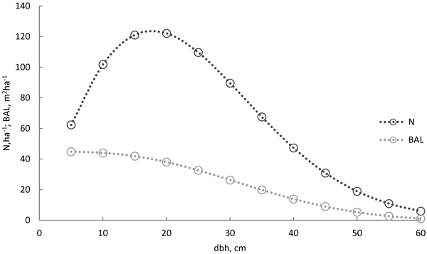
Fig. 1. The diameter distribution for the Norway spruce survival model evaluation was calculated using the model by Siipilehto and Mehtätalo (2013), based on the average characteristics of the old-growth stand (stand basal area 38 m2 ha–1, number of stems 1010 ha–1, basal area weighted mean diameter 30 cm, and age 150 years). Trees (○) were sampled for 5-cm classes, and basal-area-in-larger trees (BAL) was calculated for the sampled trees.
The model differences were illustrated using bar plots for the observed and predicted survival rates with respect to stem diameter (Monserud and Sterba 1999). Eq. 5 without stand age and the best performing alternative model with age variable were additionally evaluated using the datasets for the managed (HARKAS) and unmanaged old-growth stands (old-growth dataset). The latter evaluation was made to test the hypothesis that senescence promoted tree mortality especially in the largest diameter classes.
3 Results
3.1 Alternative individual tree survival models
The initial forms of the alternative models for tree survival are given in Eqs. 4–8. All the variables shown in Tables 2 and 3 were statistically highly significant. The best performing powers p1 and p2 differed between Eqs. 7 and 8. In Eq. 7, powers p1 and p2 were 1.8 and 0.8, while in Eq. 8, they were 1.4 and 0.9 respectively (Table 3). The dummy variable for the thinnings carried out six to 10 years ago (Thinn6_10) was statistically significant, but the dummy variable for the first five years following thinnings (Thinn5) was not.
| Table 2. The estimated logistic models for Norway spruce survival without stand age (Eq. 4, Eq. 5). | ||||||
| Eq. 4 | Eq. 5 | |||||
| Variable | estimate | std | t value | estimate | std | t value |
| Intercept | 5.4896 | 0.1413 | 38.8 | 7.1545 | 0.139 | 51.5 |
| 1/d | –2.1721 | 0.2199 | –9.88 | |||
| BAL | –0.09364 | 0.0014 | –66.4 | |||
| BAL/√(d) | –0.2844 | 0.0042 | –67.2 | |||
| d | 0.2693 | 0.0080 | 33.8 | 0.03613 | 0.0075 | 4.84 |
| d2 | –0.00673 | 0.0002 | –36.6 | –0.00206 | 0.0002 | –10.6 |
| Thinn6_10 | 0.3231 | 0.0826 | 3.91 | 0.2927 | 0.0826 | 3.54 |
| Variance | 0.6908 | 0.1173 | 5.89 | 0.7403 | 0.1238 | 5.98 |
| –2 log-likelihood | 39 794 | 39 384 | ||||
| AIC | 39 808 | 39 396 | ||||
| BIC | 39 825 | 39 410 | ||||
| Rank | 5 | 4 | ||||
| d; breast height diameter (cm) of a tree; BAL; basal area (m2 ha–1) of trees larger than the subject tree; Thinn6_10; dummy for thinnings carried out between 6 and 10 years ago (0 = unthinned, 1 = thinned). Rank; the order of fit statistics from the smallest (1 = the best fit) to the highest (5 = the worst fit) for all models. | ||||||
| Table 3. The estimated logistic models for Norway spruce survival with stand age (Eq. 6, Eq. 7, and Eq. 8). | |||||||||
| Eq. 6 | Eq. 7 | Eq. 8 | |||||||
| variable | estimate | std | t value | estimate | std | t value | estimate | std | t value |
| intercept | 7.4445 | 0.1092 | 68.2 | 7.5515 | 0.1121 | 67.4 | 7.327 | 0.146 | 50.2 |
| BAL/√(d) | –0.2856 | 0.0031 | –91.2 | –0.2898 | 0.0032 | –89.1 | –0.294 | 0.0034 | –86.1 |
| d2(Age/100) | –0.00098 | 0.00006 | –16.7 | ||||||
| d1.8(Age/100)0.8 | –0.00234 | 0.0001 | –16.2 | ||||||
| d1.4(Age/100)0.9 | –0.01079 | 0.0007 | –15.5 | ||||||
| Age/100 | 0.4124 | 0.1158 | 3.56 | ||||||
| Thinn6_10 | 0.2812 | 0.0826 | 3.41 | 0.2755 | 0.0826 | 3.34 | 0.2796 | 0.0826 | 3.38 |
| Variance | 0.7543 | 0.1263 | 5.97 | 0.7621 | 0.1275 | 5.98 | 0.7154 | 0.12 | 5.96 |
| –2 log-likelihood | 39 346 | 39 342 | 39 335 | ||||||
| AIC | 39 356 | 39 352 | 39 347 | ||||||
| BIC | 39 368 | 39 364 | 39 362 | ||||||
| Rank | 3 | 2 | 1 | ||||||
| d; breast height diameter (cm) of a tree; BAL; basal area (m2 ha–1) of trees larger than the subject tree; Thinn6_10; dummy for thinnings carried out between 6 and 10 years ago (0 = unthinned, 1 = thinned). Rank; the order of fit statistics from the smallest (1 = the best fit) to the highest (5 = the worst fit) for all models. | |||||||||
Models without stand age (Eqs. 4 and 5) had considerably poorer fit statistics (i.e. higher –2 log-likelihood, AIC, and BIC), and they therefore had a lower rank (ranks 5 and 4 respectively) (Table 2) compared with the models that included the stand age (Table 3). Eq. 6 (rank 3) and Eq. 7 (rank 2) had almost the same fit statistics (Table 3). Eq. 8, which included the interaction term between d and Age, and the independent effect Age in addition to the powers p1 and p2, was ranked the best model (Table 3). All the estimated variances (s2u 0.69–0.76) showed slight under-dispersion.
We also tested dummy variables separating the different subsets of the data, such as Naturalness for the Finnish old-growth forests and Norway dummy for the Norwegian experiments. They were not statistically significant (P = 0.65 and 0.98 respectively), denoting that survival behaved similarly in terms of the stand age and competition status of trees in the different datasets.
3.2 Evaluation results
For a wide variety of diameters, the survival probability was quite similar, despite the model (Figs. 2 and 3). Differences between models were visible in large trees. The survival probability of the largest trees (d = 55 cm) was 2% when using Eq. 4, but as high as 75% when using Eq. 5 (Fig. 2). For models including stand age, the survival probability was also very low (3%) according to Eq. 6 (Fig. 3), but considerably higher (19%) according to Eq. 7. The squared stem diameter (d2) in Eq. 6 resulted in a more rapid decrease in the survival probability for large trees than d1.8 in Eq. 7 (Fig. 3). The most plausible behaviour was provided by Eqs. 7 and 8 (Fig. 3). The difference between these two models was that the increasing age always decreased the survival probability for all size classes in Eq. 7, but in Eq. 8, the survival probability for the smaller trees was higher in an older stand compared with a younger stand with a similar diameter distribution, i.e. the survival probability curves of different stand ages crossed each other (Fig. 3). In a 100-year-old stand, the largest trees had a high survival probability (94–96%) according to Eqs. 7 and 8 (Fig. 3), but the probability decreased with increasing stand age. In a 250-year-old stand, the survival probability for a 55-cm tree increased from 19% to 40% for the following 5-year period, using Eq. 7 or 8 respectively. The powers p1 = 1.4 and p2 = 0.9 in Eq. 8 therefore reduced the effect of increasing stem diameter and age on the survival probability more than powers p1 = 1.8 and p2 = 0.8 in Eq. 7.
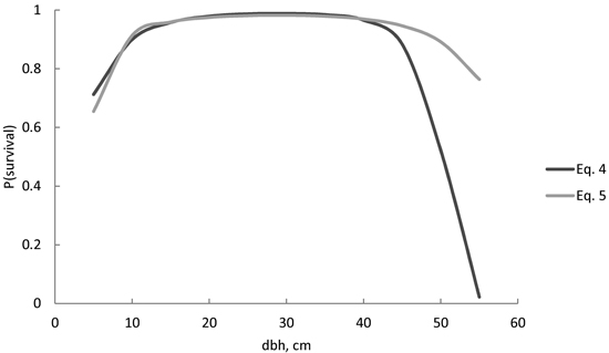
Fig. 2. Predicted Norway spruce survival probability (P) for the following 5-year period, using Eq. 4 and Eq. 5. Neither model included stand age as a predictor variable.
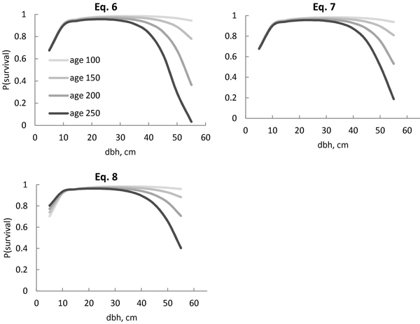
Fig. 3. Predicted Norway spruce survival probability (P) for the following 5-year period with the models (Eqs. 6–8), including interaction between age and stem diameter. The stand age ranged from 100 years (age 100) to 250 years (age 250). Eq. 8 also included stand age per se as a predictor variable, allowing intersecting curves.
All the models predicted the survival probability well for small and middle-sized trees, but they tended to underestimate survival probability for the largest trees (Fig. 4). This was partly because the survival probability in the 45–49 cm diameter class was significantly higher than in the previous 40–44 cm class. However, the number of observations was low in diameter classes above 40 cm. The differences between the survival probabilities in Eqs. 6 and 7 were small in different diameter classes (Fig. 4), as were the differences in their fit statistics (Table 3). The least underestimation was provided by Eq. 8 (Fig. 4), as well as the best statistical fit (Table 3).
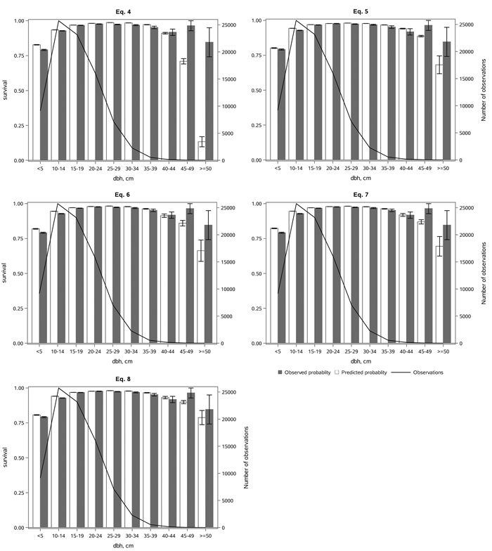
Fig. 4. The observed and predicted Norway spruce survival rate (with standard errors) by diameter classes (dbh), and the number of observations by diameter class, using the alternative models (Eqs. 4–8) in the whole dataset. View larger in new window/tab.
Eq. 5 without an age variable provided a reasonable fit in the whole dataset (Fig. 4). However, due to the formulation of Eq. 5, it could provide only an average decrease in the survival probability for large trees without a senescence effect. It was therefore not surprising that Eq. 8 fitted the subsets of the data which had a large difference in stand age much better (Fig. 5). On the managed HARKAS plots, there was hardly any mortality in the largest diameter classes. On the other hand, the survival rate in the smallest diameter classes was higher in the old-growth stands than on the managed HARKAS plots. Eq. 8 performed well in both subsets of the data (Fig. 5). However, no significant differences between the performance of Eqs. 5 and 8 were found in the Norwegian dataset, which had a maximum age of 148 years.
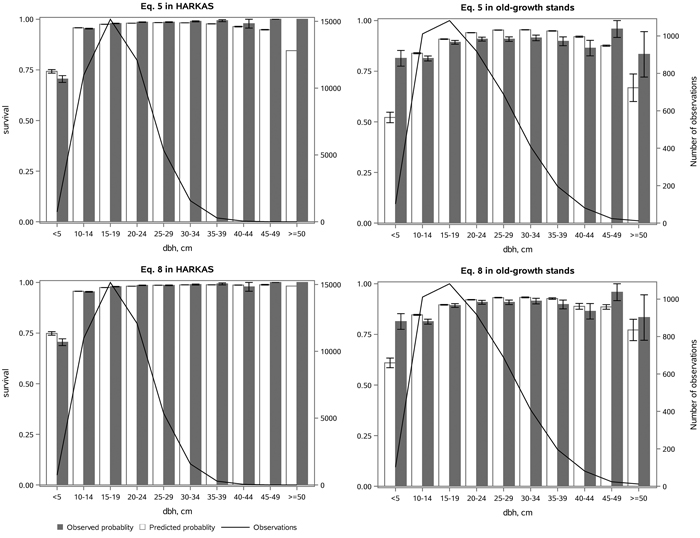
Fig. 5. The observed and predicted Norway spruce survival rate (with standard errors) by diameter class (dbh) estimated with Eq. 5, without stand age, and Eq. 8, which included the effect of age interaction with stem diameter on the tree survival, as well as the number of observations in each diameter class. The subfigures represent the HARKAS dataset, comprising both managed and unmanaged plots, and the old-growth forest stand dataset. View larger in new window/tab.
4 Discussion
The results of this study show that the senescence effect should be taken into account when modelling tree mortality for Norway spruce. The senescence effect is especially important when dealing with a combination of managed and unmanaged stands, in which trees of a certain size may differ greatly in age, depending on the past development of a stand (Henttonen et al. 2019). Indeed, the largest trees may be vigorous if their large diameter is the result of intensive thinnings, not old age.
In most datasets, the age of individual trees is typically unknown. However, stand age as the average age of dominant trees provides an effective way to account for the effect of senescence on tree survival. Although the study’s forests have been unmanaged for a long period, it is likely that the dominant individuals were regenerated after a severe natural disturbance or human activity (e.g. a slash-and-burn cultivation harvest). We therefore do not believe the use of stand age characterising tree ages to be a problem, especially as the models focus on depicting the mortality of the largest and oldest trees. Smaller trees in unmanaged stands, on the other hand, are less affected by stand age, which is a less relevant variable for them in the model.
Monserud and Sterba (1999) used a squared diameter (d2) in their model for Norway spruce in Austria, as did Yao et al. (2001) and Vieilledent et al. (2009) in their models for conifer and broadleaved species in Canada and Switzerland. Actually, the original model by Monserud and Sterba (1999) did not predict such a sudden decrease in survival rate for the largest trees as Eq. 4 in our data. Due to the large variation in the mean age in our dataset, we used the interaction of stem diameter and stand age to account for the age-dependent increasing mortality rate of the largest trees. During model development, the interaction d2 × (Age/100) proved to have a marked effect on predicted survival rates. We therefore looked for alternative powers to improve model fit and behaviour (dp1 and (Age/100)p2). This resulted in the exponents 1.8 and 1.4 for stem diameter, and 0.8 and 0.9 for age, i.e. as d2 × (Age/100), d1.8 × (Age/100)0.8, and finally, d1.4 × (Age/100)0.9. Because the exponents, p1 and p2, were lower than the corresponding powers in Eq. 6, they enabled higher survival rates for the largest trees in the old stands when using Eq. 7, and especially when using Eq. 8.
In Eq. 8, which had the best fit, the survival probability curves intersected each other. The survival probability of the smaller and intermediate trees was slightly higher in the older stands than younger stands with the same stand structure. This may be the result of increasing spacing between trees and declining resource use efficiency later in stand development (Binkley 2004). Decreasing the water and nutrient use efficiency of the largest trees (Ryan and Yoder 1997; Tyree 2003) may reduce their level of dominance in an older stand, and they may not suppress smaller trees as much as more vigorous trees of a similar size in younger stands. It is also likely that these stands have mortality events that create space for smaller trees.
The stand development classes in our dataset range from young stand some years after canopy closure to old-growth forests. The average and maximum ages of the Finnish old-growth stands were 159 and 290 years respectively. Kuuluvainen et al. (2002) found that in an old-growth forest in Russian Karelia close to Finland the oldest Norway spruce was 286 years old, while the oldest pine was as much as 525 years old. Slightly older 325-year-old spruce trees have been found in old-growth forests in Sweden (Steijlen and Zackrisson 1986; Hofgaard 1993). Norway spruce larger than 50 cm are rarely found in boreal old-growth forests in the Nordic countries (Linder 1998; Siitonen et al. 2000; Kuuluvainen et al. 2002; Rouvinen and Kuuluvainen 2005). This study’s dataset can therefore be regarded as covering the whole age and diameter range from young to old-growth stands (Henttonen et al. 2020), but not necessarily as a representative sample, because the locations of the experiments and plots were subjectively selected. We found that tree survival did not differ between the used datasets (HARKAS, the Norwegian dataset, and old-growth stands). We are therefore confident that the best fitting models are capable of predicting the survival probability for a wide range of management regimes (old-growth, unmanaged, and managed Norway spruce-dominated stands) and geographical locations.
Thinning plays a contradictory role in tree survival. On the one hand, thinning decreases between-tree competition, thereby increasing survival probability. Moreover, diameter distribution changes due to thinning, which results in changes in the basal area of larger trees (BAL). The effect of thinning on tree survival is therefore partly accounted for by using the BAL variable. On the other hand, before adapting to new conditions after thinning, trees are exposed to wind and snow damage (Valinger and Pettersson 1996; Nykänen et al. 1997; Suvanto et al. 2019). Probably due to this two-sided effect, the first five years following thinning showed no significance, whereas six to 10 years since the last thinning significantly increased survival probability. The additional effect of thinning accounts for the removal of the weakest trees with supressed tree crowns.
In the initial model adopted from Monserud and Sterba (1999), crown ratio was used to indicate tree vigour, i.e. survival probability. Unfortunately, crown size was not available in our datasets. However, it is probable that the variables for thinnings at least partly account for the relationship between the crown ratio and stand management regime. Moreover, tree vigour can be characterised by its growth rate (Monserud 1976; Yao et al. 2001; Yang and Huang 2013). However, it is laborious to measure, and the growth rate is therefore rarely available when applying the models, especially in datasets from temporary plots. Instead, we used other tree-level characteristics such as tree dbh and BAL to describe tree vigour and between-tree competition within a stand.
In conclusion, stand age appeared to play a role in the tree-level regular mortality of Norway spruce. Senescence should therefore be considered when modelling tree survival. Although our study was restricted to Norway spruce, the effect of senescence probably exists in other tree species too (Yao et al. 2001). In future studies, our intention is therefore to test if the relationship between senescence and survival probability is similar for less shade-tolerant tree species such as Scots pine and birch. Because the best model (Eq. 8) seems to perform well regarding longer rotations, we recommend it to be implemented in the decision-support tools in the Nordic countries.
Acknowledgements
This study was funded by Natural Resources Institute Finland (Luke) and Norwegian Institute of Bioeconomy Research (NIBIO). Jouni Siipilehto and Kjell Andreassen were partially funded by Nordic Forest Research (SNS) project “SNS-122_ Improving Simulation tools for assessing the long-term responses of forest carbon storage to forest management alternatives in Nordic countries”. Mikko Peltoniemi was partially funded by BiodivClim ERA-Net Cofund (Academia of Finland, decision no. 344722). We thank the anonymous reviewers for helping us to improve the manuscript.
References
Bianchi S, Siipilehto J, Hynynen J (2020) How structural diversity affects Norway spruce crown characteristics. For Ecol Manage 461: 1–9. https://doi.org/10.1016/j.foreco.2020.117932.
Binkley D (2004) A hypothesis about the interaction of tree dominance and stand production through stand development. For Ecol Manage 190: 265–271. https://doi.org/10.1016/j.foreco.2003.10.018.
Cajander AK (1925) The theory of forest types. Acta For Fenn 29. https://doi.org/10.14214/aff.7192.
Eid T, Tuhus E (2001) Models for individual tree mortality in Norway. For Ecol Manage 154: 69–84. https://doi.org/10.1016/S0378-1127(00)00634-4.
Eid T, Øyen B-H (2003) Models for prediction of mortality in even-aged forest. Scand J For Res 18: 64–77. https://doi.org/10.1080/0891060310002354.
Fridman J, Ståhl G (2001) A three-step approach for modelling tree mortality in Swedish forests. Scand J For Res 16: 455–466. https://doi.org/10.1080/02827580152632856.
Goldstein H (1995) Multilevel statistical models. Kendall’s Library of Statistics 3, 2nd edition.
Henttonen HM, Nöjd P, Suvanto S, Heikkinen J, Mäkinen H (2019) Large trees have increased greatly in Finland during 1921–2013, but recent observations on old trees tell a different story. Ecol Indic 99: 118–129. https://doi.org/10.1016/j.ecolind.2018.12.015.
Henttonen HM, Nöjd P, Suvanto S, Heikkinen J, Mäkinen H (2020) Size-class structure of the forests of Finland during 1921–2013; a recovery from centuries of exploitation, guided by forest policies. Eur J For Res 139: 279–293. https://doi.org/10.1007/s10342-019-01241-y.
Hett JM, Loucks OL (1976) Age structure models of balsam fir and eastern hemlock. J Ecol 64: 1029–1044. https://doi.org/10.2307/2258822.
Hofgaard A (1993) Structure and regeneration patterns in a virgin Picea abies forest in northern Sweden. J Veg Sci 4: 601–608. https://doi.org/10.2307/3236125.
Hosmer DW, Lemeshow S (1989) Applied logistic regression. John Wiley and Sons, New York. ISBN 0-471-61553-6.
Hynynen J, Eerikäinen K, Mäkinen H, Valkonen S (2019) Growth response to cuttings in Norway spruce stands under even-aged and uneven-aged management. For Ecol Manage 437: 314−323. https://doi.org/10.1016/j.foreco.2018.12.032.
Isomäki A, Niemistö P, Varmola M (1998) Luonnontilaisten metsien rakenne seurantakoealoilla. [The structure of natural forests on monitoring plots]. In: Annila E (ed) Monimuotoinen metsä. Metsäluonnon monimuotoisuuden tutkimusohjelman väliraportti. Metsäntutkimuslaitoksen tiedonantoja 705. Vantaan tutkimuskeskus. [In Finnish]. http://urn.fi/URN:ISBN:951-40-1647-5.
Jutras S, Hökkä H, Alenius V, Salminen H (2003) Modeling mortality of individual trees in drained peatland sites in Finland. Silva Fenn 37: 235–251. https://doi.org/10.14214/sf.504.
Kuuluvainen T, Penttinen A, Leinonen K, Nygren M (1996) Statistical opportunities for comparing stand structural heterogeneity in managed and primeval forests: an example from boreal spruce forest in southern Finland. Silva Fenn 30: 315–328. https://doi.org/10.14214/sf.a9243.
Kuuluvainen T, Karjalainen L, Lehtonen H (2002) The age distribution in old-growth forest sites in Vienansalo wilderness, eastern Fennoscandia. Silva Fenn 36: 169–184. https://doi.org/10.14214/sf.556.
Laarmann D, Korjus H, Sims A, Stanturf JA, Kiviste A, Körster K (2009) Analysis of naturalness and tree mortality patterns in Estonia. For Ecol Manage 258: 187−195. https://doi.org/10.1016/j.foreco.2009.07.014.
Linder P (1998) Structural changes in two virgin boreal forest stands in central Sweden over 72 years. Scand J For Res 13: 451–461. https://doi.org/10.1080/02827589809383006.
Mäkinen H, Isomäki A (2004) Thinning intensity and growth of Norway spruce stands in Finland. Forestry 77: 349–364. https://doi.org/10.1093/forestry/77.4.349.
Manion PD (1991) Tree disease concepts. Prentice Hall, Engelwood Cliffs, NJ, USA. ISBN 013930701X.
Monserud R (1976) Simulation of forest tree mortality. For Sci 22: 438–444.
Monserud R, Sterba H (1999) Modelling individual tree mortality for Austrian forest species. For Ecol Manage 113: 109–123. https://doi.org/10.1016/S0378-1127(98)00419-8.
Monserud R, Ledermann T, Sterba H (2005) Are self-thinning constraints needed in a tree-specific mortality model? For Sci 50: 848–858.
Nilsson SG, Niklasson M, Hedin J, Aronsson G, Gutowski JM, Linder P, Ljungberg H, Mikusinski G, Ranius T (2003) Erratum to “Densities of large living and dead trees in old-growth temperate and boreal forests”. For Ecol Manage 178: 355–370. https://doi.org/10.1016/S0378-1127(03)00084-7.
Nykänen M-L, Peltola H, Quine C, Kellomäki S, Broadgate M (1997) Factors affecting snow damage of trees with particular reference to European conditions. Silva Fenn 31: 193–213. https://doi.org/10.14214/sf.a8519.
Peltoniemi M, Mäkipää R (2011) Quantifying distance-independent tree competition for predicting Norway spruce mortality in unmanaged forests. For Ecol Manage 261: 30–42. https://doi.org/10.1016/j.foreco.2010.09.019.
Rouvinen A, Kuuluvainen T (2005) Tree diameter distributions in natural and managed old Pinus sylvestris-dominated forest. For Ecol Manage 208: 45–61. https://doi.org/10.1016/j.foreco.2004.11.021.
Ruiz-Benito P, Lines ER, Gómez-Aparicio L, Zavala MA, Coomes DA (2013) Patterns and drivers of tree mortality in Iberian forests: climatic effects are modified by competition. PLoS One 8, article id e56843. https://doi.org/10.1371/journal.pone.0056843.
Ryan MG, Yoder BY (1997) Hydraulic limits to tree height and tree growth. BioScience 47: 235–242. https://doi.org/10.2307/1313077.
Siipilehto J, Mehtätalo L (2013) Parameter recovery vs. parameter prediction for the Weibull distribution validated for Scots pine stands in Finland. Silva Fenn 47: 1–22. https://doi.org/10.14214/sf.1057.
Siipilehto J, Siitonen J (2004) Degree of previous cutting in explaining the differences in diameter distributions between mature managed and natural Norway spruce forests. Silva Fenn 38: 425–435. https://doi.org/10.14214/sf.410.
Siitonen J, Martikainen P, Punttila P, Rauh J (2000) Coarse woody debris and stand characteristics in mature managed and old-growth boreal mesic forests in southern Finland. For Ecol Manage 128: 211–225. https://doi.org/10.1016/S0378-1127(99)00148-6.
Sims A, Mändma R, Laarman D, Korjus H (2014) Assessment of tree mortality on Estonian Network of Forest Research Plots. Forestry Studies | Metsanduslikud Uurimused 60: 57–68. https://doi.org/10.2478/fsmu-2014-0005.
Steijlen I, Zackrisson O (1986) Long-term regeneration dynamics and successional trends in a northern Swedish coniferous forest stands. Can J Bot 65: 839–848. https://doi.org/10.1139/b87-114.
Suvanto S, Peltoniemi M, Tuominen S, Strandström A, Lehtonen A (2019) High-resolution mapping of forest vulnerability to wind for disturbance-aware forestry. For Ecol Manage 453, article id 117619. https://doi.org/10.1016/j.foreco.2019.117619.
Tyree MT (2003) Hydraulic limits on tree performance: transpiration carbon gain and growth of trees. Trees 17: 95–100. https://doi.org/10.1007/s00468-002-0227-x.
Tyrell LE, Crow TR (1994) Structural characteristics of old-growth hemlock-hardwood forests in relation to age. Ecology 75: 370–386. https://doi.org/10.2307/1939541.
Valinger E, Pettersson N (1996) Wind and snow damage in thinning and fertilization experiment in Picea abies in southern Sweden. Forestry 69: 25–33. https://doi.org/10.1093/forestry/69.1.25.
Vanclay J (1994) Modelling forest growth and yield. Applications to mixed and tropical forests. CAB International.
Vieilledent G, Courbaud Kunstler G. Dhote JF, Clark JS (2009) Biases in the estimation of size-dependent mortality models: advantages of a semiparametric approach. Can J For Res 39: 1430–1443. https://doi.org/10.1139/X09-047.
Wykoff WR (1990) A basal area increment model for individual conifers in the northern Rocky Mountains. For Sci 36: 1077–1104.
Yang Y, Huang S (2013) A generalized mixed logistic model for predicting individual tree survival probability with unequal measurement interval. Forest Science 59: 177–187. https://doi.org/10.5849/forsci.10-092.
Yao X, Titus SJ, MacDonald SE (2001) A generalized logistic model of individual tree mortality for aspen, white spruce, and lodgepole pine in Alberta mixedwood forests. Can J For Res 31: 283–291. https://doi.org/10.1139/x00-162.
Yli-Kojola H (2005) Metsikkö- ja puutuhojen ennustemallit. [Prediction models for stand- and tree-level damages]. Metsäntutkimuslaitoksen tiedonantoja 948. http://urn.fi/URN:ISBN:951-40-1989-X.
Young DJN, Stevens JT, Earles JM, Moore J, Ellis A, Jirka AL, Latimer AM (2017) Long-term climate and competition explain forest mortality patterns under extreme drought. Ecol Lett 20: 78–86. https://doi.org/10.1111/ele.12711.
Total of 46 references.
