Oiva Hiltunen  ,
Ville Hallikainen,
Teijo Palander
,
Ville Hallikainen,
Teijo Palander
Analysing the groundwater level and its determinants in a drained peatland forest: a case study in South Lapland, Finland
Hiltunen O., Hallikainen V., Palander T. (2023). Analysing the groundwater level and its determinants in a drained peatland forest: a case study in South Lapland, Finland. Silva Fennica vol. 57 no. 1 article id 10752. https://doi.org/10.14214/sf.10752
Highlights
- Mineral subsoils under a peat layer (less than 1 m) affect the groundwater level
- During average precipitation, silty subsoil often makes groundwater level remain too high for timber haulage
- If the subsoil is sandy and the peat layer is thin, the groundwater level gets lower
- The amount of stand evapotranspiration alone is not enough to keep the groundwater level low enough.
Abstract
In southern Lapland, 70% of drained peatland forests have a peat layer thickness of less than one metre. On these sites, the question is how the subsoil under the peat affects groundwater level and thus timber harvesting. The aim of this study was to investigate the effect of the peat layer (<1 m) and subsoil on the groundwater level and its variation during the growing season (non-frost) by modelling the factors affecting water level. In sandy soils, the groundwater level rose by 20 cm when the peat layer thickness increased from 20 to 70 cm. In silty soils the effect of the peat thickness on groundwater remained minor. When the subsoil was sand or coarser, the groundwater level was usually deeper than when it was silty or finer. The effect of stand volume (m–3 ha–1) on the groundwater level was rather weak albeit significant. The model explained a significant part of the groundwater surface variation, with a marginal coefficient of determination (R2) of 68%. It seems that the rutting of roads could be avoided in late summer if the precipitation is remarkably lower during that period, or if the subsoil is sandy with thin peat layer on top of it. Because the groundwater level affects the load-bearing capacity of timber-harvesting machinery, it is important to study this issue in more detail in the future.
Keywords
peatland;
groundwater level;
load-bearing capacity;
subsoil
-
Hiltunen,
Lapland University of Applied Sciences, Jokiväylä 11, FI-96300 Rovaniemi, Finland
E-mail
oivah@student.uef.fi
- Hallikainen, Natural Resources Institute Finland, Ounasjoentie 6, FI-96300 Rovaniemi, Finland E-mail ville.hallikainen@luke.fi
-
Palander,
The University of Eastern Finland, Faculty of Science, Forestry and Technology, P.O. Box 111, FI-80101 Joensuu, Finland
 https://orcid.org/0000-0002-9284-5443
E-mail
teijo.s.palander@uef.fi
https://orcid.org/0000-0002-9284-5443
E-mail
teijo.s.palander@uef.fi
Received 15 May 2022 Accepted 19 March 2023 Published 23 March 2023
Views 53363
Available at https://doi.org/10.14214/sf.10752 | Download PDF

1 Introduction
Investments in the forestry industry and the increased use of wood by existing mills in southern Lapland require round wood procurement from drained peatland forests all year around. Harvesting of these forests is usually done when soils are frozen. Due to climate change, as winters shorten, there is a need to increase wood harvesting during the summer (non-frost). According to the Finnish Meteorological Institute, since 2000, the temperature sum in Finland has been above the average of the period 1971–2000 almost every year (Ruosteenoja et al. 2016).
A total of 22% of the forest land in southern Lapland is peatland (National Forest Inventory (NFI) 11 2019). Drained peatlands are 70% moderately rich or poor pine-dominated forest types (Vaccinium vitis-idea type, dwarf-shrub type and Cladina type) (Hiltunen and Palander 2020). Seventy percent of the peat layer has a thickness of less than 1 m. The most fertile drained peatland forests (herb-rich type and V. myrtillus type) are mainly in the so-called Lapland Triangle (the southwestern part of southern Lapland). The peatlands forests are typically (46%) young stands (Luonnonvarakeskus 2019), which are at the stage of first commercial thinning. There are a total of 90 000 hectares of overdue thinning felling (NFI 11 2019), which is 35% of the wood production area of peatlands (Hiltunen and Palander 2020), and this area will increase in the coming years (Luonnonvarakeskus 2019). Thinning of young forests is generally low yielding, and for peatlands is even lower, due to a larger age distribution of trees and the smaller size of the trunks. Timber harvesting is already challenging in South Lapland’s peatland. Furthermore, shortening winters will increase the resource problems of industrial wood procurement, the storage costs of timber and the seasonality of timber procurement (Väätäinen et al. 2010; Palander et al. 2012).
The biggest challenge in summer harvesting is the poor load-bearing capacity of machinery on peatland soils. In addition to equipment, the load-bearing capacity is affected by the properties of peat, the amount of wood, the groundwater level and the undergrowth (Högnas et al. 2009, 2011; Uusitalo and Ala-Ilomäki 2013; Uusitalo et al. 2015). The groundwater level varies significantly during the wood procurement year, affected by the total evapotranspiration of trees and undergrowth, precipitation, runoff, and the functionality of ditches. The amount of stand evapotranspiration depends on trees´ size and vigour (Sarkkola et al. 2010; Haahti et al. 2012). According to Sarkkola et al. (2013a), the evapotranspiration of the forest keeps the water surface at a level of 30–40 cm during the growing season if the stand volume in northern Finland (where southern Lapland is located) exceeds 150 m3 ha–1 and the ditches are in a satisfactory condition. If the stand volume is less than 100 m3 ha–1, as in southern Lapland (average: 69 m3 ha–1 of all development classes), evapotranspiration is not enough to maintain the groundwater level below the level of 30–40 cm (Sarkkola et al. 2013a, 2013b). When the total evapotranspiration remains low, the functionality of the ditch network is emphasized (Haahti et al. 2012). According to Heikurainen (1957) and Hökkä et al. (2020), the ditch depth will be reduced by 20–34 cm in the 20 years. Lauhanen and Ahti (2000) reported that ditches to a depth of 1 m will shallow 40–50 cm in 14–26 years in northern Finland. Furthermore, in Lapland the climate is humid, and only 30–40% of the annual precipitation evaporates (Vakkilainen 2016).
Increasing and retaining tree growth has been the primary objective of ditching and its maintenance operations in drained peatland forests. The groundwater level – and thus the bearing capacity – is affected by the functionality of the ditch network. In this respect, the amount of ditch network maintenance in the last decade has been considerably lower than it should have been, according to NFI 11 (Hiltunen and Palander 2020). Concerns about runoff waters and their effects on water systems have contributed to this decision (nutrients, particles, heavy metals and acidity) (Nieminen et al. 2010; Hökkä et al. 2016). Further, climate concerns about drainage (greenhouse gas emissions from peat decomposition) have received more attention (Ojanen 2015). This has led to reconsidering the original idea of carrying out ditching maintenance operations. Instead of systematic and immediate ditch maintenance operations, the groundwater level would preferably be controlled by adjusting wood harvesting so that the evapotranspiration by trees would lower the ground water level, which is needed for sufficient forest growth (Sarkkola et al. 2013a; Leppä et al. 2020). It seems that the evapotranspiration by forest trees alone is not enough to keep the groundwater level low in Lapland (Sarkkola et al. 2013a, 2013b). Therefore, the ground water level remains permanently high and, consequently, the load-bearing capacity is low in peatlands, which further increases the challenges of summer harvesting.
It is known that the physical properties of the mineral soil under peat are different from those of the peat (Huikari 1959b; Päivänen 1973, 1989; Kesäniemi 2009; Ronkainen 2012). Presumably, the physical properties of the subsoil also influence the groundwater level of the thin peat soil. However, we do not know how much different mineral soil types affect the groundwater level in thin peat soil. Because water level fluctuations during the growing season have an impact on the load-bearing capacity of peat soils, it would be important to understand this phenomenon accurately. Thereafter, researchers of forest technology could develop alternative approaches to securing timber harvesting despite water level fluctuations. When the water level is sufficiently low, i.e., 30 to 40 cm, the load-bearing capacity is high enough and damage (rutting) is reduced (Högnas et al. 2009, 2011). Otherwise, new approaches are needed for cost-efficient and environmentally friendly wood procurement.
The above studies have focused on peat soils where the thickness of the peat was about 1 m or more. In southern Lapland, however, 70% of the peatland forests have a peat layer of less than 1 m. This study investigates the effect of the properties of thin peat (less than 1 m) and the soil under peat on the water level and its variation during the growing season. The study models the factors affecting the water level and discusses the meaning of the results for forest management, as well as their implications for wood procurement.
2 Materials and methods
2.1 Study area
The study area (5.8 ha) is in southern Lapland in Rovaniemi (Fig. 1). The average temperature sum of the area in 1991–2020 was 979 dd (degree days). The Finnish Meteorological Institute produces grid data for climate analysis. Grid data refer to an evenly spaced grid with an accuracy of 10 km × 10 km. For example, the temperature value is calculated in each grid using the kriging interpolation method (Finnish Meteorological Institute pages). The research site has a grid point 2911 (hereafter Hirvas) (ETRS-TM35ENG 7371916, 424857), from which the average daily temperatures and precipitation were calculated based on the calculated daily data (Table 1) and accumulated weekly precipitation during the growing season in 2017 and 2019 (Table 3). At that grid point, the temperature sum in 2017 was 875 dd and in 2019 966 dd. Between June–August, 89% of the temperature sum was generated in 2017 and 85% in 2019.
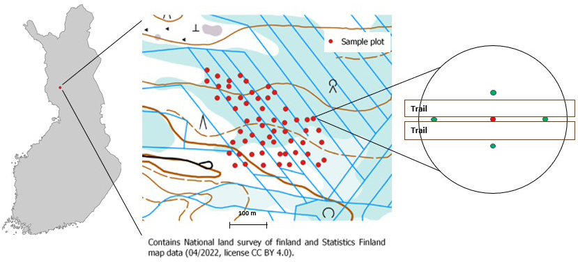
Fig. 1. Map of Finland showing the location of the research site where the sample plots were established on the drained peatland forest (ETRS-TM35FIN 7368023,425587). On the sample plot (radius: 9 m), the red dot in the middle of the strip road is the centre of the plot and the excavation by which the peat type, the degree of peat decomposition and the mineral soil type were identified. The water level was measured weekly. The green dots are the measurement points for the thickness of the peat layer; the thickness measurement was also performed from the centre of the plot.
When selecting the research site, the aim was to select a typical drained peatland forest in southern Lapland from the perspective of summer harvesting (thinning) (Hiltunen and Palander 2020). The altitude of the research site was taken into account by determining sample plots´ height above sea level (in m). According to the area-based approach (ABA) laser scanning data, the stand volume of the site varied between 90 and 200 m3 ha–1 (Uusitalo et al. 2017). The site was drained in the late 1960s to early 1970s, with the ditch spacing ranging from 37 to 49 m. Defined according to the NFI 11 classification guidelines, the condition of the ditches was “below average” or “poor” (Korhonen 2009). In this respect, the site is part of the catchment area of the then-drained bog. The plot determinations made in May–June 2017 at the site were carried out in such a way that the measured data could be used in load-bearing studies of peat soils.
| Table 1. Total precipitation and mean air temperature for June to August in 2017 and 2019 and long-term averages (2000–2019). The data for Hirvas have been calculated using the kriging interpolation method. | ||||
| Month, Annual | June | July | August | Annual |
| Precipitation (mm) | ||||
| Hirvas 2017 | 56 | 81 | 54 | 490 |
| Hirvas 2019 | 86 | 14 | 97 | 572 |
| Rovaniemi 2000–2019 | 64 (19–125) | 79 (15–152) | 70 (7–178) | 639 (422–874) |
| Temperature (°C) | ||||
| Hirvas 2017 | 11.8 | 15.6 | 12.8 | 1.7 |
| Hirvas 2019 | 13.7 | 14.8 | 13.4 | 1.6 |
| Rovaniemi 2000–2019 | 12.5 | 16.1 | 13.4 | 1.8 |
2.2 Sampling design and measurements
The research material was collected from 58 plots (Fig. 1). The circular sample plots (radius 9 m) were marked with numbered pegs. The centres were in the middle of the 16 m × 16 m (ABA) square (Fig. 1). We used stratified sampling when dividing the plots into three categories by their volume: 90–120 m3 ha–1 (group one), 120–150 m3 ha–1 (group two) and 150–180 m3 ha–1 (group three). Stand volumes were defined based on 16 m × 16 m squares. An equal number of plots in classes was a target, but it was not reached due to uneven distribution of the stand volume (a total of 25, 17 and 17 plots in groups 1, 2 and 3, respectively).
Prior to thinning, the stand volume in the plots was measured in June 2017. Sample trees with a diameter at breast height of 6 cm or more were measured. Every third tree for each tree species was chosen as a sample tree, for which the tree height and crown height were measured. Based on the sample trees, a height curve was drawn for tree species according to Näslund’s (1936) model. The volume of the trees was calculated by tree species according to the volume model of Laasasenaho (1982), based on breast height diameter and height.
The area was thinned at the end of August 2017. After felling, it was re-measured in late August/early September 2017. For defining the 2019 growing stock, the effect of the strip road area was deducted from the sizes of the plots. Thus, the results obtained for 2019 describe the stand volume outside the road. When calculating the surface area of the strip road, the average vehicle path width was used in all sample plots. The width was measured and calculated following the Finnish Forest Centre’s field inspection guidelines (Leivo et al. 2016).
The thickness of the peat layer was calculated as the average of five measurements taken within each plot (Fig. 1). The peat decomposition rate was determined from a hole in the centre of the plot (0 to 30 cm deep) according to von Post’s classification (Laine and Vasander 2008). Peat was classified as wooden-sphagnum (LS-t) or wooden-carex (LC-t) based on the plant residue composition (Laine and Vasander 2008). The depth of the ditch was measured as the distance between the bottom and the edges from the centre of the ditch. The depth of the ditch was measured below the moss layer.
| Table 2. Thickness of peat layer, volume of stand, depth of ditch and degree of decomposition of peat according to the type of mineral soil under the peat layer. The soil types are saSi = clay silt, siHkMr = silt sandy moraine, HkMr = sand moraine, srHkMr = gravel sand moraine, Hk = sand. | |||||||||||||
| Soil | N | Peat layer, cm | Volume of stand, m3 ha–1 | Depth of ditch, cm | Degree of decomposition of peat | ||||||||
| Mean | Min | Max | Mean | Min | Max | Mean | Min | Max | Mean | Min | Max | ||
| saSi | 5 | 49 | 41 | 57 | 102 | 45 | 174 | 28 | 23 | 34 | 4.0 | 2 | 7 |
| siHkMr | 12 | 42 | 23 | 70 | 110 | 40 | 181 | 36 | 20 | 44 | 4.7(10) | 3 | 7 |
| HkMr | 25 | 40 | 27 | 70 | 108 | 11 | 181 | 40 | 19 | 55 | 2.9(22) | 1 | 5 |
| srHkMr | 4 | 38 | 21 | 53 | 85 | 23 | 133 | 42 | 13 | 52 | 2.0 | 2 | 5 |
| Hk | 7 | 38 | 26 | 61 | 92 | 55 | 158 | 42 | 18 | 56 | 3.0 | 2 | 5 |
The water table level within plots was measured weekly during the growing seasons in 2017 and 2019. The water level, i.e., the distance between the surface of the peat and the water surface, was measured manually once a week to the nearest 1 cm from an excavation hole. The diameter of the hole was about 30 cm because it has been found to smooth out changes in precipitation and runoff due to its large water storage capacity (Heikurainen 1971) and the depth was about 50–60 cm. In 2017, the measurements started on 28 June and ended on 16 August (Table 3). After that, the water level in some of the plots was lower than the bottom of the excavation, so no accurate measurement result was obtained. At the beginning of June, the water level was between 0and 10 cm. Table 3 show the average groundwater levels of the plots belonging to the soil types below the peat layer on the measurement days.
| Table 3. The average groundwater levels (in cm) on measurement days according to soil types in 2017 and 2019. Precipitation is the sum of the precipitation in the week preceding the measurement. The soil types are saSi = clay silt, siHkMr = silt sandy moraine, HkMr = sand moraine, srHkMr = gravel sand moraine, Hk = sand. | ||||||||||
| Year 2017 | ||||||||||
| Soil | Group | N | 28. June | 6. July | 12. July | 20. July | 27. July | 3. Aug | 10. Aug | 16. Aug |
| saSi | Silty | 5 | 14 | 14 | 18 | 13 | 20 | 20 | 26 | 28 |
| siHkMr | Silty | 12 | 15 | 16 | 25 | 16 | 26 | 28 | 36 | 39 |
| HkMr | Sandy | 25 | 18 | 19 | 36 | 20 | 36 | 38 | 44 | 46 |
| srHkMr | Sandy | 4 | 16 | 16 | 27 | 18 | 27 | 27 | 36 | 34 |
| Hk | Sandy | 7 | 20 | 23 | 36 | 24 | 36 | 38 | 43 | 41 |
| Rain, mm | 29 | 26 | 5 | 34 | 5 | 22 | 10 | 12 | ||
| Year 2019 | ||||||||||
| Soil | Group | N | 19. June | 26. June | 3. July | 10. July | 17. July | |||
| saSi | Silty | 5 | 18 | 14 | 18 | 21 | 27 | |||
| siHkMr | Silty | 11 | 17 | 14 | 19 | 24 | 34 | |||
| HkMr | Sandy | 25 | 28 | 19 | 30 | 37 | 47 | |||
| srHkMr | Sandy | 3 | 22 | 16 | 22 | 26 | 38 | |||
| Hk | Sandy | 7 | 28 | 23 | 31 | 36 | 44 | |||
| Rain, (mm) | 19 | 37 | 11 | 6 | 4 | |||||
| Rain = Previous week’s rainfall | ||||||||||
| N = Number of plots | ||||||||||
In 2019, water level measurements began on 19 June and the water level could be observed at all test areas until 17 July (Table 3). After that, the water level in some of the plots was lower than the bottom of the excavation, so no accurate measurement was obtained, and thus the average groundwater level of the soil-type plots could not be calculated. In 2019, there were two fewer measurement points; these were damaged during timber harvesting at the end of August 2017. However, measurement was continued to find out at what point the water level rose back above 40 cm. In 2019, the last water level measurement was on September 10.
2.3 Determining the type of soil under the peat
Soil types were determined following two different approaches (Fig. 2). In the field, mineral soil samples taken from the centre of the sample plots and right under the peat layer were categorized according to the classification principles of soils for construction purposes (RT) (Jääskeläinen 2014), which is similar to the classification used in agriculture and forestry (Aaltonen et al. 1949). In the field, soil types were determined based on sensory observations (Geologian tutkimuskeskus 2005). Based on the field analysis, an additional sample was taken from 28 plots for more detailed laboratory analysis. Here, the samples were categorized according to the geotechnical soil classification (GEO) (Jääskeläinen 2014). The soil classification of each remaining plot (25 were categorized in the field) changed according to the geotechnical classification, as a more detailed analysis was provided according to that classification. According to the geotechnical classification, silt and fine sand are categorized with silt (Silty), and coarse sand belongs to sand (Sandy). In five plots, the soil type under the peat could not be determined due to the thickness of the peat.
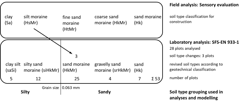
Fig. 2. Soil sample analyses and classification. First, a sensory evaluation (RT) was made in the field for all 53 plots. Second, for control purposes, 28 samples from the important groups of silt moraine and fine sand moraine were further analysed in the laboratory. This was done to ensure that the demarcation of samples between Silty and Sandy groups was correct in further analyses. Three soil samples were redirected over the critical demarcation line (grain size: 0.063 mm). Finally, soil samples were placed into revised soil types (GEO), which were further divided into Silty and Sandy groups using the Mann–Whitney U-test.
The granularity of the mineral soil was determined in accordance with the SFS-EN 933-1 standard (n = 28). To determine the granularity, the moraine samples were subjected to washing screening plus a hydrometric test or a hydrometric test alone. In the washing screen, the finest granules (0.063 mm) were first washed out of the dried and weighed sample, after which the coarser final material was dry screened. The grain size distribution of the fine material with a grain size of less than 0.063 mm was determined by a hydrometric test. The hydrometric test is based on the Stokes law. The water permeability coefficient k (m s–1) was calculated from the samples. Based on field and soil laboratory determinations, the soil types under peat were classified into five soil types: clay silt (saSi), silty sand moraine (siHkMr), sand moraine (HkMr), gravelly sand moraine (srHkMr) and sand (Hk) (Table 2).
2.4 Statistical analysis
We used the Mann–Whitney U-test to determine differences in water levels between groups. This test is suitable for small independent observations, and the distributions of the comparative groups do not have to be in accordance with the normal distributions (Metsämuuronen 2006; Tähtinen et al. 2020). The soil types belonging to the Sandy group had no difference in the water surface averages in the measurements of different measurement periods. Similarly, there was no difference between the soil types within the Silty group. When we compared water level averages between the two groups (Sandy and Silty), the difference was either statistically significant (p < 0.01) or very significant (p < 0.001), and the effect size was moderate (r = 0.30) or strong (r = 0.50). The Silty group (n = 17 plots, grain size < 0.063 mm) encompassed the clay silt (saSi) and silt sand moraine (siHkMr) soil types, whereas the Sandy group (n = 36 plots, grain size > 0.063 mm) encompassed the sand moraine (HkMr), gravelly sand moraine (srHkMr) and sandy (Hk) types. Five plots for which the soil type under peat could not be identified due to the thickness of the peat were excluded from the analysis.
A linear mixed-effects model (Gaussian family) was constructed to explain (more than predict) the groundwater level. The response variable (groundwater level) was log-transformed to normalize the distribution and achieve reasonable residuals. The hierarchy of the model consisted of the random year effect, the measurement point effect measured within the two years and the repeated measurements of each measurement point during the calendar weeks (lowest level observations). The repeated measurements mean the repeatedly done measurements from the plots. The repeated measurements in a certain calendar year were numbered from 1 to 8. Two years were taken in the same model and were interpreted as “random blocks” although they were temporal in nature. The model is as follows:
![]()
where ln(yijk) denotes the log-transformed response variable, groundwater level, in year i and measurement point j and measurement number (or calendar week) k. Further, f() denotes a linear function with arguments Xijk (i.e., fixed predictors, measured from the levels ijk), and β (i.e., fixed parameters). Term μi denotes the random year effect, μij the measurement point effects within the years and normally distributed error variance with AR (1) correlation structure. The AR (1) was needed because several repeated measurements within measurement points could be expected to be correlated in time, the adjacent measurements being more correlated than measurements distant in time. Thus, the temporal autocorrelation term (phi) was estimated in the model. The compound symmetry correlation structure was assumed for the random year effect and for the measurement points.
The models were built using the 11 candidate fixed predictors mentioned in Table 4. The stages of the model construction were as follows. First, the contribution of the single predictors was tested in the model. All variables that indicated at least a slight contribution were considered as possible candidates in the following stages. This denoted that p-values should be at 0.050 or at least near that level. Second, all the variables were forced into the same model, and their contribution and collinearities (variance inflation factor, VIF) were checked in the forced main effects model. Third, the main effects and all their possible two-way interactions were checked. Fourth, the final significant (about a 5% risk level) main effects and their interaction were selected for the “technical” version of the model candidate. Fifth, the meaning of all the possible fixed explanatory variables, as well as their interactions, were evaluated. All the variables and their interactions had to be environmentally reasonable or generally known (according to former studies, e.g., Hökkä et al. 2008) as important to the groundwater level. The VIF values of the main effects of the explanatory variables (together in the model) were < 5. Thus, the multicollinearity was not a serious problem in the random years model.
We also computed a model using year as the fixed effect. However, the random year alternative was selected instead of fixed year because of the simpler model structure (less interactions) and the goal of generalization. This means that the predictions were computed using fixed predictors (marginal, population-level predictions). In addition, the model with a fixed year suffered more considerable multicollinearity problems (highest VIF values being about 7.5).
All analyses were made in the R statistical environment (R Core Team 2016). The R package nlme and its function lme (Pinheiro et al. 2017) were used to model the groundwater level. The coefficients of determination (R2) were computed for the model using the R package MuMIn (Bartoń 2017). The fixed effects predictions with their 95% confidence intervals for the model were calculated and plotted using the R package effects (Fox 2003).
3 Results
The thickness of the peat layer ranged from 21 to 70 cm and the average was 41 cm (Table 2). Table 4 shows the characteristics of the distributions of the continuous and categorical variables and the variables’ frequencies and ratios for both groups, Silty and Sandy. The peat of the Sandy group was on average poorly decomposed (Table 2) and had an average thickness of 40 cm. The peat of the Silty group was on average moderately decomposed (Table 2) and had an average thickness of 44 cm. There were no statistical differences in stand volume between silty and sandy plots in 2017 (p = 0.175; 135 vs. 124 m3 ha–1) nor after thinning in 2019 (p = 0.588; 80 vs. 84 m3 ha–1). However, the stand volumes varied from 11 to 181 m3 ha–1 (Table 4). There was no statistical difference in the depth of the ditches between the groups (p = 0.230). In Silty soils the mean depth of the ditch (34 cm) was slightly lower than in Sandy soils (38 cm), and the range was larger than in Silty soils. Further, the depth of the ditch ranged from 13 to 56 cm.
| Table 4. Tested explanatory variables for the linear mixed effects model. The parameters of distributions (continuous variables) or the frequencies (numbers of observations in the longitudinal data) and the proportions of the categories (categorical variables) are presented in the table. | ||||
| Variable | Mean | Median | Minimum | Maximum |
| Continuous variables: | ||||
| Groundwater level, cm (response) | 27.35 | 24.00 | 8.00 | 65.00 |
| Volume of stock, m3 ha–1 | 108.20 | 111.60 | 10.50 | 181.00 |
| Measurement, nr. | 3.93 | 4.00 | 1.00 | 8.00 |
| Rainfall (during week), mm | 16.89 | 12.00 | 3.70 | 37.20 |
| Temperature (during day), °C | 14.04 | 13.90 | 10.20 | 16.90 |
| Peat decomposition, scale 1–8 | 3.34 | 3.00 | 1.00 | 7.00 |
| Altitude, m a.s.l. | 83.02 | 82.83 | 80.40 | 86.64 |
| Ditch depth, cm | 35.82 | 35.00 | 13.00 | 56.00 |
| Depth of peat layer, cm | 41.44 | 39.00 | 21.00 | 70.00 |
| Categorical variables: | ||||
| Peat type | wooden-sphagnum peat: 85% (515), wooden-carex peat 15% (91) | |||
| Mineral soil type | Silty: 31% (190), Sandy: 69% (416) | |||
The explanatory variables were tested in the modelling of the groundwater level (Table 5), and the statistically significant variables at a 5% risk level with significant two-way interactions were included in the model. Ditch depth was not statistically significant at a 5% risk level, but it was taken into account in the model because of its theoretical importance and the generally known importance of the modelled phenomena – e.g., Hökkä et al. (2008).
| Table 5. Parameter estimates and tests of a general linear mixed effects model (Gaussian) for the groundwater level. Std. err. denotes the standard error of the estimates, df denotes the degrees of freedom, t-values are the test values for the parameter estimates, and p is the statistical significance level. R2 for the marginal model was 68.4% and that for the conditional model was 81.4%. | |||||
| Variable | Coefficient | Std. err. | df | t-value | p |
| Fixed effects: | |||||
| Intercept | 13.791 | 4.905 | 511.000 | 2.812 | 0.005 |
| Peat type, carex-sphagnum peat, ref. wooden-carex peat | –0.155 | 0.064 | 83.000 | –2.412 | 0.018 |
| Volume of timber stock, m3 ha–1 | 0.002 | 0.001 | 83.000 | 2.973 | 0.004 |
| Rainfall (during the period week), mm | –0.014 | 0.001 | 511.000 | –26.370 | 0.000 |
| Measurement, nr | 0.083 | 0.005 | 511.000 | 16.044 | 0.000 |
| Mineral soil type, sandy, ref. silty | 1.110 | 0.233 | 83.000 | 4.761 | 0.000 |
| Depth of peat layer, cm | –0.367 | 0.134 | 83.000 | –2.748 | 0.007 |
| Ditch depth, cm | 0.003 | 0.002 | 83.000 | 1.928 | 0.057 |
| Altitude, m.o.s.l. | –0.133 | 0.060 | 83.000 | –2.220 | 0.029 |
| Mineral soil type*Depth of peat layer | –0.025 | 0.006 | 83.000 | –4.105 | 0.000 |
| Depth of peat layer*Altitude | 0.004 | 0.002 | 83.000 | 2.713 | 0.008 |
| Random effects (variances) and phi (AR1 correlation structure), 95% confidence limits in the parenthesis: | |||||
| Random year effect | 1.509e-2 (0.079e-2–0.289) | ||||
| Random sample point effect | 1.354e-2 (0.593e-2–3.092e-2) | ||||
| Residual | 4.092e-2 (3.206e-2–5.223e-2) | ||||
| Phi | 0.511 (0.377–0.623) | ||||
Peat type affected the groundwater level. The predicted groundwater level in wooden-sphagnum type peat was 21.7 cm and the level in wooden-carex peat was 25.3 cm when the values of the other explanatory variables were fixed at their mean values (continuous variables) or average levels (categorical variables). When the stand volume increased, the groundwater level decreased – that is, the groundwater was deeper in places with abundant trees. Further, the effect could be rather weak as the range (confidence intervals) of the estimates for the parameter was large (Fig. 3a). In contrast, increasing rainfall during the period increased the groundwater level – that is, the groundwater was closer to the surface. Fig. 3b shows that the groundwater level increased more than 10 cm when the rainfall increased from 5 to 40 mm during the period. Furthermore, the effect of the summer period on the groundwater level was also noticeable (Fig. 3c): the groundwater was about 15 cm deeper at the last measurement at the end of the summer (August) compared to the first measurement in early summer (June).
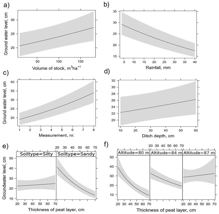
Fig. 3. The predictions of the continuous explanatory variables and their interactions for the ground water level model by predictors: volume of tree stock (a), rainfall (b), number of measurements during a growing season (c), ditch depth (d) and the interaction of soil type and ditch depth (e), altitude and thickness of peat layer (f). The predicted groundwater level values for the fifth (categorical) predictor variable peat type were: wooden-sphagnum type peat 21.7 cm and wooden-carex peat 25.3 cm. The other explanatory variables were fixed at their mean values (continuous variables) or at their average levels (for categorical variables, see Table 4).
Increased ditch depth caused a deeper groundwater level, but the p-value of the parameter estimate was 0.057 (Table 5). The thickness of the peat layer affected the groundwater level differently depending on the mineral soil type. In Silty soils, an increase in the peat layer slightly increased the groundwater level, but the confidence intervals suggested that the increase could be caused by chance (Fig. 3e). However, in the Sandy soils, the groundwater level was 20 cm higher when the peat layer was 70 cm than when it was 20 cm thick (Fig. 3e). Also, the measurements (Table 3) show that the groundwater level was lower in the soil types of the Sandy group than in the Silty group. Fig. 3f shows that the thickness of the peat layer affected the groundwater level in the lowest places in the study area (altitude about 80 m above sea level), but in the highest places, no effects between the depth of peat layer and groundwater level were observed (altitude of 87 m above sea level). The p-value of interaction between altitude and peat depth estimate was 0.008 (Table 5).
The model statistics indicate that the variance for the two years was slightly bigger than the variance for the measurement points, but the confidence intervals for the variance estimate for the random year effect were considerably larger. The adjacent repeated measurements were rather strongly correlated over time (phi about 0.5, Table 5). The linear predictors explained a remarkable proportion of the variation in the groundwater level, the marginal coefficient of determination (R2) being about 68%. In addition, Fig. 4 suggested that the residuals of the model were fair and no serious systematic bias was found. Furthermore, the observed and predicted values were fairly in line with each other, observing the predicted and residual values in the log-transformed scale. The mean values in the original scale were also close to each other, the observed being 27.4 cm and the predicted 27.1 cm.
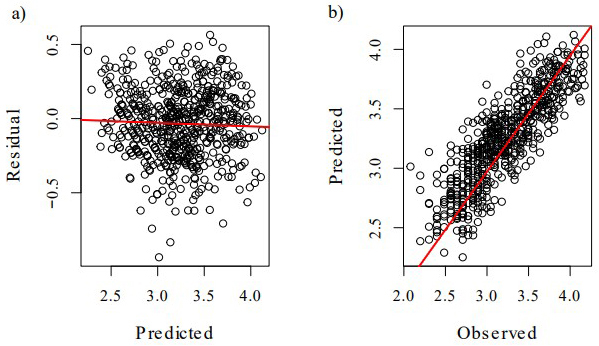
Fig. 4. Scatter plots for the predicted values vs. residuals (a) and observed vs. predicted values (b) of the model in the log-transformed scale. The values were computed using the fixed part of the model (marginal model).
4 Discussion
We investigated the effect of peat type, amount of wood stock in forest, and the subsoil under the peat on the groundwater level and its variation during the growing season in a drained peatland forest with a thin layer of peat (less than 1 m). In a thin peat layer, the physical properties of the subsoil under the peat are different from those in the peat. Further, the physical properties of different mineral soil types are different. Therefore, we assumed that the soil type influences the water level of the peat. This assumption was examined by modelling the factors affecting water level. We also address the phenomenon because it relates to wood procurement conditions during the summer.
4.1 Determinants of ground water level
The groundwater level was systematically lower in the sample plots with mineral soil belonging to the Sandy group (Table 3). Further, on the sandy soil, as the thickness of the peat layer increased, the groundwater level increased (Fig. 3e). The peat was, on average, poorly decomposed, in which case the water-retention capacity of peat was high due to its low density and large pore volume (Huikari 1959a; Päivänen 1973; Kesäniemi 2009). As the tension of the groundwater increases (rainless period), the poorly decomposed peat releases water relatively easily. Considering the higher water permeability of Sandy soils compared to peat, the result is – as the study showed – that the change in water level is faster and quantitatively larger than with Silty soils. Again, this is related to the high water-retention capacity and slower water permeability of Silty soils. In peat on top of Silty soil, the movement of water is more in a horizontal direction towards the ditch than vertically, in the depth direction (Hökkä et al. 2021). In the Silty plots, the peat was, on average, moderately decomposed, which further slowed down the movement of water in the peat (Päivänen 1973).
As the thickness of the peat layer increased, it had a stronger effect on groundwater level in the Sandy soil group compared to the Silty group. Actually, the level of groundwater was almost the same in the Silty group regardless of the thickness of the peat layer (Fig. 3e). Therefore, our assumption was justified that the subsoil type influences the water level of the peat. Previous studies have shown that, as the thickness of peat increases, its decay and density increase, which has a detrimental effect on water permeability and at the same time increases water retention (Huikari 1959a; Päivänen 1973; Kesäniemi 2009). It follows that the infiltration of water into peat layers is considerably slower than in a thin and poorly degraded peat layer. That is, the properties of the peat, such as thickness, affected the most on the groundwater level in the Sandy soil type group. In other words, the thicker the peat layer, the less the subsoil type will affect the groundwater level.
In this study when the total stand volume increased by 25 m3 ha–1, the decrease in groundwater level was 1 cm (derived from Fig. 3a). This is less than half of what Sarkkola et al. (2010) found in their study, which was 1 cm/10 m3 ha–1. On the other hand, Haahti et al. (2012) found that, in northern Finland, the water surface depth decreased by 1 cm as the basal area increased by 4.7 m2 ha–1. Using a 4.7 m2 ha–1 basal area and the average height of the trees means that an increase in stand volume of 28 m3 ha–1 will lower the water level by 1 cm. Based on this, the difference in water level between the smallest and largest stand volume of sample plots would be 6 cm, which corresponds to the results obtained. When the functioning of the ditch network is inadequate or poor, as at the study site, even high stand volumes (m3 ha–1) alone is not sufficient to keep the groundwater level low enough for the proper growth of trees. In addition, given the poor drainage efficiency of the ditches, the water level may remain too high (30–40 cm) for maximum growth of trees during July and August, as suggested by Sarkkola et al. (2010, 2013). In the 2019 growing season, July and the beginning of August were the driest times of the review period (2000–2019) (Table 1). Therefore, the water level dropped so low that it could not be determined weekly at the end of the growing season (Table 3).
According to the results, the ditch impact on the groundwater remained small (Table 5). Although the depth of ditches was satisfactory in places, the bases of ditches were covered with abundant moss and were partially clogged. This may have a detrimental effect on the drying capacity of the ditch network (Heikurainen 1957, 1980; Päivänen 1989; Silver and Joensuu 2005). There was not statistical difference in the depth of the ditches and the volume of stands between the Sandy and Silty groups. Similarly, the condition of the ditches was similar in both groups. So, it may be assumed that the groundwater level in the Silty group soil remains higher than in the Sandy group due to the properties of the Silty mineral soil and peat, and partly due to the altitude (Fig. 3f). The water flow (runoff) also depends on the slope of the peatland (Päivänen 1989).
4.2 Implications for wood procurement
For successful summer wood harvesting, it is necessary to know the carrying capacity of the peatland. On sandy soils, the thickness of the peat layer has a great impact on the groundwater level, unlike on silty soils (Fig. 3e). Information on the thickness of the peat layer and the type of soil under it allows for more accurate wood procurement planning and implementation, which also results in decreased harvesting damage and costs. Finally, the results suggest that – unlike in the existing classification for southern Finland (Högnas 2011) – the effect of the peat thickness and the mineral soil type under peat should be included in the wood procurement classification system to be developed for northern Finland.
In the study area in 2017 and 2019, the groundwater level of individual plots varied widely. The minimum variation was 22 cm (5–27 cm) and the maximum variation was 54 cm (11–65 cm). In such a situation, where the water level of such a small site (5.8 ha) is permanently or partially too high in part of the area during the growing season, it makes it difficult to determine the harvestability class. According to the harvest classification by Högnas et al. (2009, 2011), during the growing seasons of 2017 and 2019, the harvest class varied between several categories. This means that only part of the site could be harvested in non-frost, depending on the groundwater level, growing stock, peat thickness, and harvesting equipment. Results suggested that rutting of roads can be avoided in two occasions. First, it could be avoided in all stands regardless of subsoil type or peat layer thickness if precipitation is remarkably lower than the average (Table 1) during that period. Second, it could also be avoided if precipitation during that period is about the average or less, and the subsoil is sandy with thin peat layer on top of it. Further, the poor water conductivity of ditches may alter the hydrological properties of peatland forests. In this case, the load-bearing capacity of the peat will change on strip roads.
The harvestability classification should aim at real-time information on the load-bearing capacity of peat. The amount of rain and its temporary variation, which can be strong, can significantly change the load-bearing capacity of peat. However, we do not know the magnitude and duration of the change in groundwater level caused by rain. It is generally estimated (intuitively or ad hoc), if the rainfall is such that harvesting should be interrupted. The amount of harvest damage is the measure used for the interruption. Studies like this provide a better understanding of the phenomenon and make it possible to react in nearly real time to changes in harvesting conditions. This would mean that, if necessary, machine operators would make the necessary changes in harvesting methods to enable work to continue and, at the same time, avoid harvesting damage and additional costs. In addition, it should be investigated how much, how fast and for how long the rainfall affects the groundwater level. Furthermore, it would be important to determine the role of cumulative rainfall over a period of time in predicting the groundwater level, and also taking the growing stock, characteristics of peat and type of subsoil into account.
5 Conclusions
The aim of the study was to investigate the effects of the properties of drained peatland on the groundwater level and its variation, in regard to stand, peat (less than 1 m) and subsoil under peat. The research material was collected in Northern Finland in a forest of Southern Lapland before and after mechanical thinning. The site represented a typical peatland forest of the area from the perspective of the functioning of the ditch network, which was in poor condition. Based on the developed regression model, the groundwater level and its variation are most affected by the thickness of the peat and the subsoil type under the peat. The thickness of peat layer affected the groundwater level only slightly when the subsoil was Silty. In contrast, the groundwater level variation was larger when the subsoil was Sandy. In practical forestry applications, this probably enables predicting water level sinking on these subsoil sites when the rainfall (mm) is also observed. Based on the results, the wood amount of the stand was too low to keep the groundwater level low, although the effect was significant. The ditch depth was not statistically significant.
The time frame for non-frost timber haulage usually sets between spring and late summer peaking water levels (melting snow, increasing rains). Yet unpredictable weather patterns pose challenges – sometimes opportunities – for effective and timely timber procurement planning in drained peatland forests. We should further increase our understanding of the temporal and spatial changes of groundwater levels in drained peatland forests. This would enable to increase the timber harvesting volume and to extend timber harvesting period towards autumn.
Acknowledgements
We are grateful to MSc (Agr. & For.) Sirkka Jokela for helping with the field analyses. We appreciate Dr (Agr. & For.) Juha-Pekka Snäkin for providing us with valuable comments during the research process. In addition, we thank Mr. Jani Norvapalo from PBM Oy Ltd. for enabling the analyses of soil samples. We further thank Lapin koulutuskeskus REDU (Lapland Education Centre REDU) and Metsähallitus for enabling research to be done out in the area. We thank MSc (Agr. & For.) Markus Korhonen and Dr (Agr. & For.) Kari Mäkitalo for giving valuable advice. Finally, the comments and suggestions of reviewers helped to improve the quality of this manuscript.
Conflict of interest statement
None declared.
Declaration on the openness of research data
The weather data used are public and available from the Finnish Meteorological Institute. Researcher’s written notes are available upon request.
Author contributions
Oiva Hiltunen: The conception of the research question and design of the work; Acquisition, analysis, and interpretation of data and results; Majority of the scientific writing of the work; Revising critically for sound intellectual content; Final approval of the version to be published.
Ville Hallikainen: Provided knowledge of statistical methods that helped with the selection of analysis and modelling; Helped with the conception of the research question; Performed the statistical analysis; Analysed the results; Revising critically for sound and intellectual content; Final approval of the version to be published.
Teijo Palander: Helped with the conception of research question and design of the work; Contextualizing results; Revising critically for sound and intellectual content; Final approval of the version to be published.
Funding
The study was funded by the Natural Resources Institute of Finland and the University of Eastern Finland.
References
Aaltonen VT, Aarnio B, Hyyppä E, Kaitera P, Keso L, Kivinen E, Kokkonen E, Kotilainen P, Sauramo M, Tuovila P (1949) Maaperäsanaston ja maalajien luokituksen tarkastus 1949. [A critical review of soil classification in Finland in the year 1949]. Maataloustieteellinen aikakausikirja 21: 37–66. https://doi.org/10.23986/afsci.71269.
Bartoń K (2017) MuMIn: multi-model inference. R package version 1.40.0. https://CRAN.R-project.org/package=MuMIn.
Fox J (2003) Effect displays in R for generalized linear models. J Stat Softw 8: 1–27. https://doi.org/10.18637/jss.v008.i15.
Geologian tutkimuskeskus (2005) Geological survey of Finland. Verkkojulkaisu ISBN 951-690-924-8 © GTK. http://weppi.gtk.fi/aineistot/mp-opas/index.htm.
Haahti K, Koivusalo H, Hökkä H, Nieminen M, Sarkkola S (2012) Vedenpinnan syvyyden spatiaaliseen vaihteluun vaikuttavat tekijät ojitetussa suometsikössä Pohjois-Suomessa. [Factors affecting the spatial variability of water table depth within a drained peatland forest stand in northern Finland]. Suo 63 :107–121. http://www.suo.fi/article/9883.
Heikurainen L (1957) Metsäojien syvyyden ja pintaleveyden muuttuminen sekä ojien kunnon säilyminen. [Changes in depth and top width of forest ditches and the maintain of their repair]. Acta For Fenn 65: 1–45. https://doi.org/10.14214/aff.7468.
Heikurainen L (1971) Pohjavesipinta ja sen mittaaminen ojitetuilla soilla. [Ground water level in drained peat soils and its measurement]. Acta For Fenn 113: 1–23. https://doi.org/10.14214/aff.7547.
Heikurainen L (1980) Kuivatuksen tila ja puusto 20 vuotta vanhoilla ojitusalueilla. [Drainage condition and tree stand on peatlands drained 20 years ago]. Acta For Fenn 167: 1–39. https://doi.org/10.14214/aff.7614.
Hiltunen O, Palander T (2020) Puuntuotannon ja puunhankinnan kehittämismahdollisuudet Etelä-Lapin ojitetuilla soilla. [The development opportunities of silviculture and wood procurement on drained peatland forests in southern Lapland]. Suo 71: 1–18. http://www.suo.fi/article/10401.
Högnas T, Kärhä K, Lindeman H, Palander T (2009) Turvemaaharvennusten kantavuusluokitus. [Load capacity classification of peatland forest thinnings]. Metsätehon tuloskalvosarja 17/2009. Metsäteho, Vantaa, Finland. https://www.metsateho.fi/wp-content/uploads/2015/02/Tuloskalvosarja_2009_17_Turvemaaharvennusten_kantavuusluokitus_kk.pdf. Accessed 19 March 2023.
Högnas T, Kumpare T, Kärhä K (2011) Turvemaaharvennusten korjuukelpoisuusluokitus. [Harvesting eligibility classification of peatland forest thinning’s]. Metsätehon tuloskalvosarja 3/2011. Metsäteho, Vantaa, Finland. http://www.metsateho.fi/wp-content/uploads/2015/02/Tuloskalvosarja_2011_03_Turvemaaharvennusten-korjuukelpoisuusluokitus_kk_th_tk.pdf. Accessed 19 March 2023.
Hökkä H, Repola J, Laine J (2008) Quantifying the interrelationship between tree stand growth rate and water table level in drained peatland sites within Central Finland. Can J For Res 38: 1775–1783. https://doi.org/10.1139/X08-028.
Hökkä H, Salminen H, Ahtikoski A, Kojola S, Launiainen S, Lehtomaa M (2016) Long-term impact of ditch network maintenance on timber production, profitability and environmental loads at regional level in Finland: a simulation study. Forestry 90: 234–246. https://doi.org/10.1093/forestry/cpw045.
Hökkä H, Stenberg L, Laurén A (2020) Modelling depth of drainage ditches in forested peatlands of Finland. Balt For 26, article id 453. https://doi.org/10.46490/BF453.
Hökkä H, Laurén A, Stenberg L, Launiainen S, Leppä K, Nieminen M (2021) Defining guidelines for ditch depth in drained Scots pine dominated peatland forests. Silva Fenn 55, article id 10494. https://doi.org/10.14214/sf.10494.
Huikari O (1959a) Kenttämittaustuloksia turpeiden veden läpäisevyydestä. [Field measurement results on water permeability of peats]. Metsäntutkimuslaitoksen julkaisuja 51: 1–26. http://urn.fi/URN:NBN:fi-metla-201207171083.
Huikari O (1959b) Metsäojitettujen turvemaiden vesitaloudesta. [On the ground water level of drained peatlands forest]. Metsäntutkimuslaitoksen julkaisuja 51: 1–45. http://urn.fi/URN:NBN:fi-metla-201207171083.
Ilmatieteen laitos (2021) [Finnish Meteorological Institute]. https://ilmatieteenlaitos.fi/terminen-kasvukausi. Accessed 30 October 2021.
Jääskeläinen R (2014) Geotekniikan perusteet. [Basics of geotechnics]. Amk-Kustannus Oy, Porvoo. ISBN 978-952-5491-50-0.
Kesäniemi O (2009) Rahkaturvemaiden hydrauliset ominaisuudet. [Hydraulic properties of peat soils]. Licentiate thesis, Helsinki University of Technology. http://urn.fi/URN:NBN:fi:aalto-202104156020.
Korhonen KT (2009) NFI 11 Maastotyöohje 2009/koko Suomi/2.painos. [Fieldwork instructions 2009/ Whole Finland/2.edition]. National Forest Inventory (NFI), Finnish Forest Research Institute (Metla). http://urn.fi/URN:NBN:fi-fe201603038534.
Laasasenaho J (1982) Taper curve and volume functions for pine, spruce, and birch. Commun Inst For Fenn 108: 1–74. http://urn.fi/URN:ISBN:951-40-0589-9.
Laine J, Vasander H (2008) Suotyypit ja niiden tunnistaminen. [Peatland types and their identification]. Metsäkustannus Oy, Karisto Oy, Hämeenlinna. ISBN 978-952-5694-20-8.
Lauhanen R, Ahti E (2000) Kunnostusojituksella kestävään suometsien kasvatukseen. [Drainage network maintenance for sustainable peatland forest management]. Metsätieteen aikakauskirja, article id 6018. https://doi.org/10.14214/ma.6018.
Leivo J, Partanen J, Nieminen T, Vuorenmaa J, Kuoppala H, Rahkola S (2016) Maastotarkastusohje. [Field Inspection instructions]. Suomen Metsäkeskus.
Leppä K, Korkiakoski M, Nieminen M, Laiho R, Hotanen J-P, Kieloaho A-J, Korpela L, Laurila T, Lohila A, Minkkinen K, Mäkipää R, Ojanen P, Pearson M, Penttilä T, Tuovinen J-P, Launiainen S (2020) Vegetation controls of water and energy balance of a drained peatland forest: Responses to alternative harvesting practices. Agric For Meteorol 295: 1–17. https://doi.org/10.1016/j.agrformet.2020.108198.
Luonnonvarakeskus (2019) [Natural Resources Institute Finland (Luke)]. TuPa hakupalvelu-NFI11–NFI12 (2013–2017). http://mela2.metla.fi/mela/tupa/index.php. Accessed 30 October 2021.
Metsämuuronen J (2006) Tutkimuksen tekemisen perusteet ihmistieteissä. [Research fundamentals for social sciences]. International Methelp ky and J Metsämuuronen, Jyväskylä. ISBN-10 952-5372-21-9.
Näslund M (1936) Skogsforsoksanstaltens gallringsförsok i tallskog. [Skogsforsoksanstalt’s thinning experiment in pine forest]. Meddelanden fran Statens Skogsforsoksanstalt häfte 29: 1–169. http://urn.kb.se/resolve?urn=urn:nbn:se:slu:epsilon-e-1187.
NFI 11 (2019) Luonnonvarakeskus. [Natural Resources Institute Finland (Luke)]. Taulukkoluettelo. Taulukot liittyvät julkaisuun Suomen metsät 2009–2013 ja niiden kehitys 1921–2013. Luonnonvara- ja biotalouden tutkimus 59/2017. [Catalog of tables. The tables relate to the publication Finnish Forests 2009–2013 and their development 1921–2013. Natural Resources and Bioeconomy Research 59/2017]. http://urn.fi/URN:ISBN:978-952-326-467-0.
Nieminen M, Ahti E, Koivusalo H, Mattsson T, Sarkkola S, Laurén A (2010) Export of suspended solids and dissolved elements from peatland areas after ditch network maintenance in south-central Finland. Silva Fenn 44: 39–49. https://doi.org/10.14214/sf.161.
Ojanen P (2015) Metsäojituksen vaikutukset ilmastoon. [Climate impacts of forestry on drained boreal peatlands]. Suo 66: 49–55. http://www.suo.fi/article/9898.
Päivänen J (1973) Hydraulic conductivity and water retention in peat soils. Acta For Fenn 129. https://doi.org/10.14214/aff.7563.
Päivänen J (1989) Suometsät ja niiden hoito. [Peatlands forests and their management]. Kirjayhtymä Oy, Helsinki. ISBN 951-26-3059-1.
Palander T, Bergroth J, Kärhä K (2012) Excavator technology for increasing the efficiency of energy wood and pulp wood harvesting. Biomass Bioenerg 40: 120–126. https://doi.org/10.1016/j.biombioe.2012.02.010.
Pinheiro J, Bates D, DebRoy S, Sarkar D, R Core Team (2017) nlme: linear and nonlinear mixed effects models. R package version 3: 1–131. https://CRAN.R-project.org/package=nlme.
R Core Team (2019) R: a language and environment for statistical computing. R Foundation for Statistical Computing, Vienna, Austria. https://www.R-project.org/.
Ronkainen N (2012) Suomen maalajien ominaisuuksia. [Properties of Finnish soil types]. Finnish Environment Institute (SYKE) Suomen ympäristökeskus, Helsinki. ISBN 978-952-11-3975-8. http://hdl.handle.net/10138/38773.
Ruosteenoja K, Räisänen J, Venäläinen A, Kämäräinen M, Pirinen P (2016) Terminen kasvukausi lämpenevässä ilmastossa. [Thermal growing season in a warming climate]. Terra 128: 3–15.
Sarkkola S, Hökkä H, Koivusalo H, Nieminen M, Ahti E, Päivinen J, Laine J (2010) Role of tree stand evapotranspiration in maintaining satisfactory drainage conditions in drained peatlands. Can J For Res 40: 1485–1496. https://doi.org/doi:10.1139/X10-084.
Sarkkola S, Hökkä H, Jalkanen R, Koivusalo H, Nieminen M (2013a) Kunnostusojitustarpeen arviointi tarkentuu – puuston määrä tärkeä ojituskriteeri. [The assessment of drainage network maintenance becomes more accurate – the volume of stands is an important ditching criterion]. Metsätieteen aikakauskirja 2: 159–166. https://doi.org/10.14214/ma.6884.
Sarkkola S, Nieminen M, Koivusalo H, Ahti E, Launiainen S, Nikinmaa E, Marttila H, Laine J, Hökkä H (2013b) Domination of growing-season evapotranspiration over runoff makes ditch network maintenance in mature peatland forests questionable. Mires and Peat 11: 1–11. http://www.mires-and-peat.net/pages/volumes/map11/map1102.php.
Silver T, Joensuu S (2005) Ojien kunnon säilymiseen vaikuttavat tekijät kunnostusojituksen jälkeen. [The condition and deterioration of forest ditches after ditch network maintenance]. Suo 56: 69–81. http://www.suo.fi/article/9839.
Tähtinen J, Laakkonen E, Broberg M (2020) Tilastollisen aineiston käsittelyn ja tulkinnan perusteita. [Basics of processing and interpreting material of statistical]. Turun yliopiston kasvatustieteiden tiedekunnan julkaisuja C. https://urn.fi/URN:ISBN:978-951-29-8091-8.
Uusitalo J, Ala-Ilomäki J (2013) The significance of above-ground biomass, moisture content and mechanical properties of peat layer on the bearing capacity of ditched pine bogs. Silva Fenn 47, article id 993. https://doi.org/10.14214/sf.993.
Uusitalo J, Salomäki M, Ala-Ilomäki J (2015) Variation of factors affecting soil bearing capacity of ditched pine bogs in southern Finland. Scand J For Res 30: 429–439. https://doi.org/10.1080/02827581.2015.1012110.
Uusitalo J, Haavisto M, Kaakkurivaara T (2017) Utilizing airborne laser scanning technology in predicting bearing capacity of peatland forest. Croat J For Eng 33: 329–337. https://crojfe.com/archive/volume-33-no-2/utilizing-airborne-laser-scanning-technology-in-predicting-bearing-capacity-of-peatland-forest/.
Väätäinen K, Lamminen S, Sirén M, Ala-Ilomäki J, Asikainen A (2010) Ympärivuotisen puunkorjuun kustannusvaikutukset ojitetuilla turvemailla – korjuuyrittäjätason simulointitutkimus. [Cost effects of year-round timber harvesting on drained peatlands – a simulation study of harvesting entrepreneur]. Working Papers of the Finnish Forest Research Institute (Metla) 184. http://urn.fi/URN:ISBN:978-951-40-2276-0.
Vakkilainen P (2016) Hydrologian perusteet. [The basics of hydrology]. In: Paasonen-Kivekäs M, Peltomaa R, Vakkilainen P, Äijö H (eds) Maan vesi- ja ravinnetalous – ojitus, kastelu ja ympäristö. Salaojayhdistys ry, Helsinki, pp 73–123. http://salaojayhdistys.fi/wp-content/uploads/2016/05/web_maanvesijaravinnetalous_B5_2016.pdf.
Total of 49 references.
