Matti Katila  ,
Tuomas Rajala,
Annika Kangas
,
Tuomas Rajala,
Annika Kangas
Assessing local trends in indicators of ecosystem services with a time series of forest resource maps
Katila M., Rajala T., Kangas A. (2020). Assessing local trends in indicators of ecosystem services with a time series of forest resource maps. Silva Fennica vol. 54 no. 4 article id 10347. https://doi.org/10.14214/sf.10347
Highlights
-
Untitled Document Contextual Mann-Kendall test detects significant trends in time-series of forest maps - Trends become more consistent as the areal unit size used for test input increases
- Changes in different scales reflect different phenomena in forests
- Significant trends were detected even after multiple testing correction.
Abstract
Since the 1990’s, forest resource maps and small area estimates have been produced by combining national forest inventory (NFI) field plot data, optical satellite images and numerical map data using a non-parametric k-nearest neighbour method. In Finland, thematic maps of forest variables have been produced by the means of multi-source NFI (MS-NFI) for eight to ten times depending on the geographical area, but the resulting time series have not been systematically utilized. The objective of this study was to explore the possibilities of the time series for monitoring the key ecosystem condition indicators for forests. To this end, a contextual Mann-Kendall (CMK) test was applied to detect trends in time-series of two decades of thematic maps. The usefulness of the observed trends may depend both on the scale of the phenomena themselves and the uncertainties involved in the maps. Thus, several spatial scales were tested: the MS-NFI maps at 16 × 16 m2 pixel size and units of 240 × 240 m2, 1200 × 1200 m2 and 12 000 × 12 000 m2 aggregated from the MS-NFI map data. The CMK test detected areas of significant increasing trends of mean volume on both study sites and at various unit sizes except for the original thematic map pixel size. For other variables such as the mean volume of tree species groups, the proportion of broadleaved tree species and the stand age, significant trends were mostly found only for the largest unit size, 12 000 × 12 000 m2. The multiple testing corrections decreased the amount of significant p-values from the CMK test strongly. The study showed that significant trends can be detected enabling indicators of ecosystem services to be monitored from a time-series of satellite image-based thematic forest maps.
Keywords
National Forest Inventory;
satellite images;
k-nearest neighbour estimation;
Landsat;
Mann-Kendall test;
multitemporal inventory data;
temporal trend analysis
-
Katila,
Natural Resources Institute Finland (Luke), Bioeconomy and environment, Latokartanonkaari 9, FI-00790 Helsinki, Finland;
 https://orcid.org/0000-0001-6946-5736
E-mail
matti.katila@luke.fi
https://orcid.org/0000-0001-6946-5736
E-mail
matti.katila@luke.fi
- Rajala, Natural Resources Institute Finland (Luke), Natural resources, Latokartanonkaari 9, FI-00790 Helsinki, Finland E-mail tuomas.rajala@luke.fi
-
Kangas,
Natural Resources Institute Finland (Luke), Bioeconomy and environment, Yliopistokatu 6, FI-80100 Joensuu, Finland
https://orcid.org/0000-0002-8637-5668
E-mail
annika.kangas@luke.fi
Received 6 April 2020 Accepted 7 September 2020 Published 14 September 2020
Views 82503
Available at https://doi.org/10.14214/sf.10347 | Download PDF

1 Introduction
National forest inventories (NFIs), provide data for natural resource management information needs in national and regional scales (Corona et al. 2011). NFIs also provide information on indicators of ecosystem condition such as the number of tree species and the stand age (Winter et al. 2011). Assessing sustainability of the forest use, however, requires time series of data rather than a snapshot from one timepoint and thus periodical data are needed.
In smaller scales, remote sensing is the only available data source supporting change monitoring. In addition, remote sensing forms an important resource in sustainable forest management, because it provides spatially explicit information on various forest attributes used as ecosystem service indicators (Haakana 2017; Vauhkonen and Ruotsalainen 2017). Czúcz and Condé (2018) list, among others, forest tree species richness, deadwood, forest age and growing stock as the key ecosystem condition indicators for forests; most of them can be assessed employing remote sensing. Rocchini et al. (2019) used a measure of spectral diversity of remote sensing images in a spatial domain as a proxy, in order to produce a time series of indicators of biodiversity. Using suitable remote sensing data, the biophysical characteristics of species’ habitats, distribution of species and spatial variability in species richness, may be identified and monitored at various scales from individual landscapes to large geographical areas (Kerr and Ostrovsky 2003). In forest management, the natural units are forest stands, forest estates, municipalities and regions or provinces.
Remote sensing data are cost-effective and readily available for forest inventory purposes (McRoberts et al. 2010; Wulder et al. 2012). The free and open access to Landsat image archives has made it possible to produce large-area pixel-based composites and their time series, capturing the temporal autocorrelation between time points (White et al. 2014; Saarinen et al. 2018). There has been a huge increase in studies using Landsat time series and many of them have focused on change detection methods (Zhu 2017). Abrupt changes can be detected by comparing images from two different time points (Pitkänen et al. 2020). Long-term decline or growth, however, requires more images and poses more challenges (Coops et al. 2020). For instance, there is variance in the image data due to seasonal differences and atmospheric variability (Gómez et al. 2011; Zhu 2017).
The Finnish multi-source NFI (MS-NFI) produces thematic maps and statistics for small areas by using NFI field plot data, optical satellite images and numerical map data. The NFI field plots are measured by following a systematic cluster sampling design. Mostly Landsat 5–8 satellite series images have been used as satellite data. A non-parametric k-nearest neighbour (k-NN) method is used in the estimation (Tomppo et al. 2008; Tomppo and Halme 2004; Mäkisara et al. 2016). Finland has the longest history of producing small-area estimates and thematic maps by means of an MS-NFI. The first operative Finnish MS-NFI results were calculated in 1990 (Tomppo 1990) and the first results for the entire country were published in 1998 (Tomppo et al. 1998). Since 2005, almost the entire country has been covered by an MS-NFI every second year. The eighth MS-NFI results (corresponding to 2015) are the latest published (Mäkisara et al. 2019) and the ninth results, MS-NFI-2017, are already available (Forest resource maps and municipal statistics 2020). This study shall employ a time series of thematic forest maps covering both abrupt and gradual changes and considering spatial domain of the data to detect significant trends.
Forest growing stock change components are the volume increment and drain (Tomppo et al. 2011). The major component of drain is removals from cuttings and natural hazards. The yearly area of intermediate and regeneration fellings covers approximately 3% of forest land (national definition) in Finland (Finnish Forest Research Institute 2014). The average size of managed stands in southern Finland is about 1.2 hectares (Parviainen and Västilä 2011). Thus, we can expect major changes in forest stands, possibly adjacent ones, over more than half of the forests available for wood production during a period of two decades. The average size of private owned forest property entities, covering three-fifths of Finland’s total forest land area, is 30.5 hectares (Luke’s Statistics database 2019). Most of the forest owners aim to manage sustainably their forest estates.
Neeti and Eastman (2011) presented a contextual Mann-Kendall (CMK) test for assessing significant trends from a time series. The CMK test is an extension of the original Mann-Kendall sign test suitable for small sample sizes (Mann 1945; Kendall 1975). It uses spatial autocorrelation to account for trends in neighboring pixels. Neeti and Eastman (2011) found the CMK test to reduce the amount of single isolated pixels with significant trends while increasing the significance of trends elsewhere when carrying out the test to mean annual normalized difference vegetation index products over 22 years in West Africa. Czerwinski et al. (2014) employed the CMK test to detect gradual and abrupt changes on a temperate mixed forests using thirteen Landsat 5 Thematic Mapper (TM) scenes from a growing season covering a 20-year time span.
A (large-scale) multiple testing problem arises from testing thousands or more pixels from geographical data simultaneously, such as thematic forest maps. Several methods to correct for multiple testing have been proposed and they differ in their ease of implementation and their stringency (Goovaerts 2010). Additionally, tests over geographical units might not be independent, so a correction which is robust against correlated tests is preferable (Benjamini and Yekutieli 2001).
The aim of this study is 1) to test whether statistically significant changes can be found on a time series of the MS-NFI thematic maps over a period of about two decades and 2) to assess the effect of spatial scale on the significance and 3) to address the multiple testing problem in the resulting large number of simultaneous statistical tests. The CMK test was employed (Neeti and Eastman 2011). The potential of the method to detect trends in the forest variables used as indicators of ecosystem services, and finally the potential of using the detected trends as indicators of sustainability is discussed.
2 Materials and methods
The study sites consist of two rectangular areas from South Finland and North Finland called Häme and Kainuu, measuring 182 × 144 km2 and 191 × 191 km2, respectively (Fig. 1). The study sites are characterized by typical boreal forests dominated by Scots pine (Pinus sylvestris L.) and Norway spruce (Picea abies (L.) Karst.). Birch (Betula spp.) and other deciduous species occur often as mixed species. Pine and spruce accounted for the largest proportion of the total volume at the Kainuu and Häme sites, respectively.
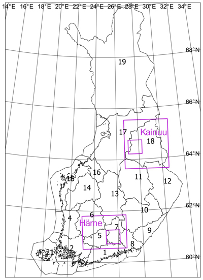
Fig. 1. The Häme and Kainuu study sites (rectangles) and two subareas within them. The regions of Finland. Digital map data: contains data from the National Land Survey of Finland general map 1:4.5 M 06/2015 and municipal division 1:4.5 M 01/2018.
2.1 Multi-Source estimates
The multi-source thematic maps used in this study are from the MS-NFI-8 (Tomppo et al. 1998), MS-NFI-9 (Tomppo et al. 2008), MS-NFI-2002 (only Häme site) (Mäkisara et al. 2001), MS-NFI-2005 (Tomppo et al. 2009), -2007 (Tomppo et al. 2012), -2009 (Tomppo et al. 2013), -2011 (Tomppo et al. 2014), -2013 (Mäkisara et al. 2016), -2015 (Mäkisara et al. 2019) and -2017 (Forest resource maps and municipal statistics 2020). NFI field plot data from four to five years time period was typically used in the MS-NFI. During the MS-NFI-8 and MS-NFI-9, the NFI progressed by region and field plots were mostly from the same year as the satellite images. Since the tenth NFI (2004–2008), one-fifth of the clusters have been measured annually in major parts of Finland. Therefore, the NFI plots from the last five years have been employed in the MS-NFI as training data since MS-NFI-2005 (Table 1). In addition to NFI field plots, the data sources behind these estimates are high-resolution multispectral satellite images with pixel sizes of about 10–30 meters (Landsat TM, ETM+ and OLI, Spot XS HRV, IRS-1 LISS–III, Sentinel-2A MSI) and digital map data of land use from the National Land Survey of Finland. The survey’s topographic database has been the digital map data source since MS-NFI-2005. The digital map data are used to separate forestry land (FRYL) from other land classes (an output is a FRYL mask) as well as to stratify FRYL and corresponding field plots into open bogs and fens, mineral soil and peatland strata for k-NN estimation purposes (Katila and Tomppo 2002; Tomppo et al. 2008).
| Table 1. The multi-source national forest inventories (MS-NFI) used, the measurement years of the training data and the mean (x̄) and the standard deviation (sd) of the mean volume maps on intersecting forestry land (FRYL) masks of the MS-NFIs on the two study sites. | |||||||
| MS-NFI | Reference | Häme c | Kainuu d | ||||
| Tr. data years | x̄ | sd | Tr. data years | x̄ | sd | ||
| m3 ha–1 | m3 ha–1 | m3 ha–1 | m3 ha–1 | ||||
| MS-NFI-8 | (Tomppo et al. 1998) | 1994 | 144.3 | 77.7 | 1990, 1992 | 56.5 | 55.6 |
| MS-NFI-9 | (Tomppo et al. 2008) | 1996–1999 | 147.0 | 78.7 | 1996, 2000–2002 | 67.0 | 55.8 |
| MS-NFI-2002 | (Mäkisara et al. 2001) | 1996–1999 a | 148.2 | 82.9 | |||
| MS-NFI-2005 | (Tomppo et al. 2009) | 1996–1999 a, 2004–2005 a | 151.7 | 80.5 | 1996 a, 2000–2002 a, 2004–2005 a | 74.4 | 54.1 |
| MS-NFI-2007 | (Tomppo et al. 2012) | 2005–2008 | 141.6 | 81.6 | 2005–2008 | 73.9 | 56.5 |
| MS-NFI-2009 | (Tomppo et al. 2013) | 2006–2010 b | 151.2 | 83.5 | 2006–2010 b | 76.2 | 54.6 |
| MS-NFI-2011 | (Tomppo et al. 2013) | 2007–2011 b | 157.5 | 84.1 | 2007–2011 b | 84.3 | 60.0 |
| MS-NFI-2013 | (Mäkisara et al. 2016) | 2009–2013 b | 163.6 | 85.3 | 2009–2013 b | 86.6 | 59.8 |
| MS-NFI-2015 | (Mäkisara et al. 2019) | 2012–2016 b | 161.7 | 96.3 | 2012–2016 b | 86.1 | 60.2 |
| MS-NFI-2017 | (Forest resource maps and municipal statistics 2020) | 2013–2017 b | 162.1 | 97.0 | 2013–2017 b | 88.8 | 66.0 |
| a Field plots computationally updated to the date of the satellite image data. b Field plots computationally updated to 31 July of the MS-NFI year. c The area of the intersecting FRYL masks was 1 394 908 ha. d The area of the intersecting FRYL masks was 2 541 772 ha. | |||||||
Multi-source predictions for the pixels on FRYL masks are weighted averages or modes of k-NN (NFI field plots) to the pixel. The weights are based on distance metrics defined in the feature space of the satellite image data and, since MS-NFI-9, the coarse scale forest variable map values have been also used as features. The weight wi,p of plot i for each image pixel p is determined by a k-NN method (Tomppo and Katila 1991) and, after MS-NFI-9, by an improved k-NN method (Tomppo and Halme 2004; Tomppo et al. 2008). The pixels that cover the centre of a field plot i belonging to the training data are called field plot pixels pi, and wi,p ≠ 0 if field plot pixel pi is among the nearest neighbours of pixel p to be predicted. The training data are restricted to the same satellite image and map stratum (mineral soils and peatlands), within a given upper limit to the geographical distance from the target pixel (Tomppo et al. 2008; Mäkisara et al. 2016). Typically, anywhere from several hundred to a few thousand NFI field plots exist on FRYL (national definition) as training data to a satellite image (Mäkisara et al. 2019). For example, 67 264 and 55 029 field plots were measured on FRYL employed across Finland in the MS-NFI-9 and MS-NFI-2015, respectively.
Thematic forest maps of the most important forest variables are produced in raster format for the MS-NFI. These include variables considered as indicators for biodiversity or provision of ecosystem services, such as proportion of broadleaved trees (which often occur as mixed species and thus increase the number of tree species) of the mean volume and stand age (Winter et al. 2011) as well as volume of growing stock and mean volume of tree species groups (forest tree species richness) (Czúcz and Condé 2018). The mean and the standard deviation of the mean volume predictions on FRYL masks are presented in Table 1 for each MS-NFI used.
2.2 Creation of maps of various unit size
The original MS-NFI thematic maps were first re-rectified, if necessary, to the ETRS-TM35FIN coordinate system (MS-NFI-2009 and prior) with a spatial resolution of 16 m by 16 m (MS-NFI-2005 and prior were originally of pixel size 25 × 25 m2 and MS-NFI-2007 – MS-NFI-2011 of pixel size 20 × 20 m2). The maps of various unit sizes were created by aggregating (i.e., calculating a mean value) the thematic maps of pixel size 16 × 16 m2 to 240 × 240 m2, 1200 × 1200 m2 and 12 000 × 12 000 m2. The unit sizes were selected to be multiplicative to both 16 m and 20 m resolutions. In this way the aggregated units followed the original MS-NFI map grids, at least for the MS-NFI-2009 and later. The smallest unit, the original pixel, represents a sub-stand scale (the average forest stand area in southern Finland is about 1.2 hectares or 110 × 110 m2), the second smallest unit represents a large stand or a group of stands, the next unit size represents a large forest estate (an average estate size is about 30 hectares or 550 × 550 m2 (Luke’s Statistics database 2019)).
The largest unit is the size of a small municipality (the smallest municipality in Häme is 125 km2 or 11 200 × 11 200 m2). For the 16 × 16 m2 pixel size maps, subareas of the study sites were used (Fig. 1) in the calculation of CMK tests due to the otherwise excessive data size if whole areas had been used. All the other land use pixels were converted to zero to avoid comparison between the FRYL mask delineation of the subsequent MS-NFIs. However, a minimum proportion of FRYL mask pixels was defined to have the following unit values: 80% for 240 × 240 m2 and 50% for 1200 × 1200 m2 and larger. Otherwise, a missing value was attached to the unit. The aggregated mean values for the units thus covered both FRYL mask and, to some extent, other land use.
2.3 The CMK test
The Mann-Kendall test examines the slopes between all pair-wise combinations of a sample and tests for a monotonic trend. The H0 is that there is no trend. The pair-wise observations are ranked with reference to time in the forward direction. The Kendall’s S is:
![]()
and
where n is the number of observations of the time series data and xi and xj are the observations at time points i and j. The S statistic is approximately normal when n ≥ 8. Without ties, the variance of S depends only on the number of observations and takes the form σ2 = VarS = n(n–1) (2n+5) / 18 (with ties additional correction term appears, see Neeti and Eastman (2011)).
The standardized Z test statistic is:
The Z statistic follows the standard normal distribution approximately. As the observations are ordered in time the statistic S is the number of pairwise comparisons where the later value is higher so a positive Z-value indicates an upward trend, for example, and a p-value for statistical significance of the trend can then be calculated using the normal cumulative distribute function.
The CMK test incorporates spatial autocorrelation, which is often present in remote sensing images and forests (Wallerman 2003), into the test statistic. The test statistic S is smoothed locally: Let Sp denote the test statistic at pixel p, and let N(p) be the neighborhood of pixels around p with n(p) = #N(p) denoting its size. Note that the pixel here represents any size of map unit used in this study. We used the 3 × 3 neighbourhood consisting of the pixel p and its 8 adjacent neighbors. Pixels at the mask edge have less neighbors accordingly. The new locally averaged test statistic is then defined as:

and its normalized version is:

To account for the correlation in the neighbouring pixels’ time series, the variance needs to be calculated as:

Here, VarSp = σ2 and the cross-covariances are computed as Cov(Sp',Sp") ![]() where
where ![]() is the sample cross-correlation coefficient of the time series at pixels p' and p".
is the sample cross-correlation coefficient of the time series at pixels p' and p".
With thousands or more pixels to test simultaneously, we must correct for the systematic increase of false positives. The problem is known in statistics as the multiple testing problem (Benjamini and Yekutieli 2001; Goovaerts 2010). Controlling the family-wise error rate (which in practice amounts to lowering the globally applied p-value threshold) by avoiding false positives is too stringent a criterion when we can assume at least some true positives to occur. We therefore applied the less conservative false discovery rate (FDR) adjustment, minimising instead the proportion of false positives. We also chose FDR as geographical units can be correlated, especially after local smoothing, and FDR allows some correlation between tests (Benjamini and Yekutieli 2001). An R (2020) package of Contextual Mann-Kendall trend test for raster image stacks was constructed and is freely available at GitHub repository (Open Geospatial Information Infrastructure for Research 2020).
3 Results
The significance of a trend in time series of various MS-NFI forest variable maps was tested on the two study sites. The primary forest variables reported in the MS-NFI (Mäkisara et al. 2019) were selected: the mean volume of growing stock, the mean volume of pine and spruce, the proportion of broadleaved tree species of the mean volume and the stand age.
The CMK test showed significant (p < 0.05) trends for mean volume of the 240 × 240 m2, 1200 × 1200 m2 and 12 000 × 12 000 m2 units at the Häme study site (51.4, 46.3 and 76.1% of the units, respectively) and at the Kainuu site (66.0, 82.0 and 99.5%, respectively). For the 16 × 16 m2 pixels in subareas of the Häme and Kainuu study sites, respective proportions of units with significant trend were 30.8% and 36.7% (Table 2). In general, the proportion of units with significant trend increased as unit size increased.
| Table 2. The proportion of units with a significant (p < 0.05) trend from the contextual Mann-Kendall test statistic and the proportion of positive S statistic in the case of significant trend. MS-NFI time series 1994–2017 (n = 10) of thematic maps at the Häme study site and 1992–2017 (n = 9) at the Kainuu study site. The mean volume, mean volumes of pine and spruce, proportion of broadleaved tree species of the mean volume and the stand age are listed variables for both sites. | |||||
| Site | Variable | 16 × 16 m2 a | 240 × 240 m2 | 1200 × 1200 m2 | 12 000 × 12 000 m2 |
| p % (of which S positive %) | |||||
| Häme | Volume (m3 ha–1) | 30.8 (81) | 51.4 (97) | 46.3 (98) | 76.1 (100) |
| pine (m3 ha–1) | 31.1 (86) | 32.5 (96) | 50.0 (100) | ||
| spruce (m3 ha–1) | 29.9 (83) | 26.3 (63) | 37.7 (44) | ||
| Prop. of broadl. spp. % | 32.0 (68) | 49.4 (95) | 79.0 (100) | ||
| Stand age (y) | 24.4 (47) | 36.2 (5) | 65.2 (0) | ||
| Kainuu | Volume (m3 ha–1) | 36.7 (92) | 66.0 (99) | 82.0 (100) | 99.5 (100) |
| pine (m3 ha–1) | 62.0 (98) | 76.5 (100) | 98.1 (100) | ||
| spruce (m3 ha–1) | 32.2 (94) | 27.7 (99) | 38.3 (100) | ||
| Prop. of broadl. spp. % | 13.7 (13) | 11.0 (11) | 4.9 (0) | ||
| Stand age (y) | 29.7 (90) | 19.7 (89) | 9.7 (100) | ||
| a Results cover a subarea of the study site (Fig. 1). | |||||
Of the other variables, the largest proportions of significant trend were found for the proportion of broadleaved trees of the mean volume in the Häme study site and for the pine volume in the Kainuu study site. The proportion of significant trend also increased with the unit size except for the proportion of broadleaved trees and the stand age at the Kainuu study site (Table 2). The sign of the S statistic for the units where significant trend was detected was counted and, for both study sites, it was positive in almost all cases. A negative trend (S < 0, Eq. 1) was detected for the Häme study site’s spruce mean volume and stand age as well as for the proportion of broadleaved trees of the mean volume at the Kainuu study site. The sign of the trend was more polarized towards positive or negative as the unit size increased.
When multiple testing correction was applied to the p-values, no significant trend was detected for the mean volume at the original pixel size, and for the other unit sizes, the proportion of significant trend decreased at both study sites (Table 3). This is partly due to the fact that the correction for p-values was stronger when the number of tests was larger (i.e., the size of the units got smaller). The trend detected by pmulti in the units was almost always positive. (Table 3). However, at the Häme site, the detected trend for spruce mean volume was negative for most cases and negative for all cases of stand age. At the Häme study site, a significant trend was found only for the largest size units when measured with pmulti < 0.05, except for the mean volume and proportion of broadleaved trees of the mean volume. At the Kainuu study site, the positive trend in pine volume was strong. For the other variables, there was no trend at any scale except for the spruce mean volume at 12 000 × 12 000 m2 resolution (Table 3). In the following results, the multiple testing corrected values (pmulti) are applied.
| Table 3. The proportion of units with significant trend, given multiple testing corrected p-values (pmulti < 0.05), from the Contextual Mann-Kendall test statistic and the proportion of positive S statistic in the case of significant trend. MS-NFI time series 1994–2017 (n = 10) of thematic maps at the Häme study site and time series 1992–2017 (n = 9) at the Kainuu study site. The mean volume, mean volumes of pine and spruce, the proportion of broadleaved tree species of the mean volume and the stand age are listed variables for both sites. | |||||
| Site | Variable | 16 × 16 m2 a | 240 × 240 m2 | 1200 × 1200 m2 | 12 000 × 12 000 m2 |
| pmulti % (of which S positive %) | |||||
| Häme | Volume (m3 ha–1) | 0 | 39.8 (98) | 26.2 (99) | 72.5 (100) |
| pine (m3 ha–1) | 0 | 0 | 37.0 (100) | ||
| spruce (m3 ha–1) | 0 | 0 | 10.1 (36) | ||
| Prop. of broadl. spp. % | 0 | 33.3 (99) | 75.4 (100) | ||
| Stand age (y) | 0 | 0 | 49.3 (0) | ||
| Kainuu | Volume (m3 ha–1) | 0 | 59.6 (99) | 79.6 (100) | 99.5 (100) |
| pine (m3 ha–1) | 54.0 (99) | 72.0 (100) | 98.1 (100) | ||
| spruce (m3 ha–1) | 0 | 0 | 6.8 (100) | ||
| Prop. of broadl. spp. % | 0 | 0 | 0 | ||
| Stand age (y) | 0 | 0 | 0 | ||
| a Results cover a subarea of the study site (Fig. 1). | |||||
A longitudinal plot of values for randomly selected units, where significant trend in the CMK test was detected, is presented for various unit sizes in Fig. 2. There is more variation in the time series for the 240 × 240 m2 units and some abrupt changes can be seen among the units with a negative trend (Fig. 2b). Nevertheless, the trends of all scales are in accordance with the sign of the S statistic. The trends become more consistent when the unit size increases, despite deviations in the time series; for instance, the MS-NFI-2007 estimates seem to deviate systematically downwards in the time series. Deviation can be seen for the Häme study site also in Table 1.
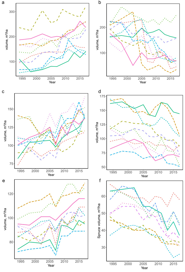
Fig. 2. A random sample of 10 units from a subset of units with significant trend (pmulti < 0.05) from the contextual Mann-Kendall test applied to time series of multi-source NFI mean volume thematic maps at the Häme study site dated 1994–2017. 240 × 240 m2 units and positive S statistic (a), 240 × 240 m2 units and negative S statistic (b), 1200 × 1200 m2 units and positive S statistic (c), 1200 × 1200 m2 units and negative S statistic (d), 12 000 × 12 000 m2 units and positive S statistic (e), mean volume of spruce, 12 000 × 12 000 m2 units and negative S statistic, 9 units (f).
Positive or negative trend with different unit sizes is visualized with the standardized Z statistic of the CMK in Fig. 3. At the original pixel size, 16 × 16 m2, the delineation of forest stands is visible. A clear decline, negative Z statistic –2.0, can be seen on areas where a regeneration cutting (which is typical for even-aged forest stands in Finland) or a removal of the major part of the growing stock has occurred between 1992 (MS-NFI-8 volume map) and 2017 (MS-NFI-2017 volume map), according to a regeneration cutting mask (grey color in Fig. 3). The regeneration cutting mask was obtained using a threshold classification of the image difference between the two MS-NFI mean volume maps on pixels that belonged to the forest mask in both images. In the 240 × 240 m2 units, the largest cutting areas are still visible as a negative Z statistic. In the larger 1200 × 1200 m2 units, single cutting areas are no longer visible, partly due to contextual information. Therefore, negative trends are rare in this scale.
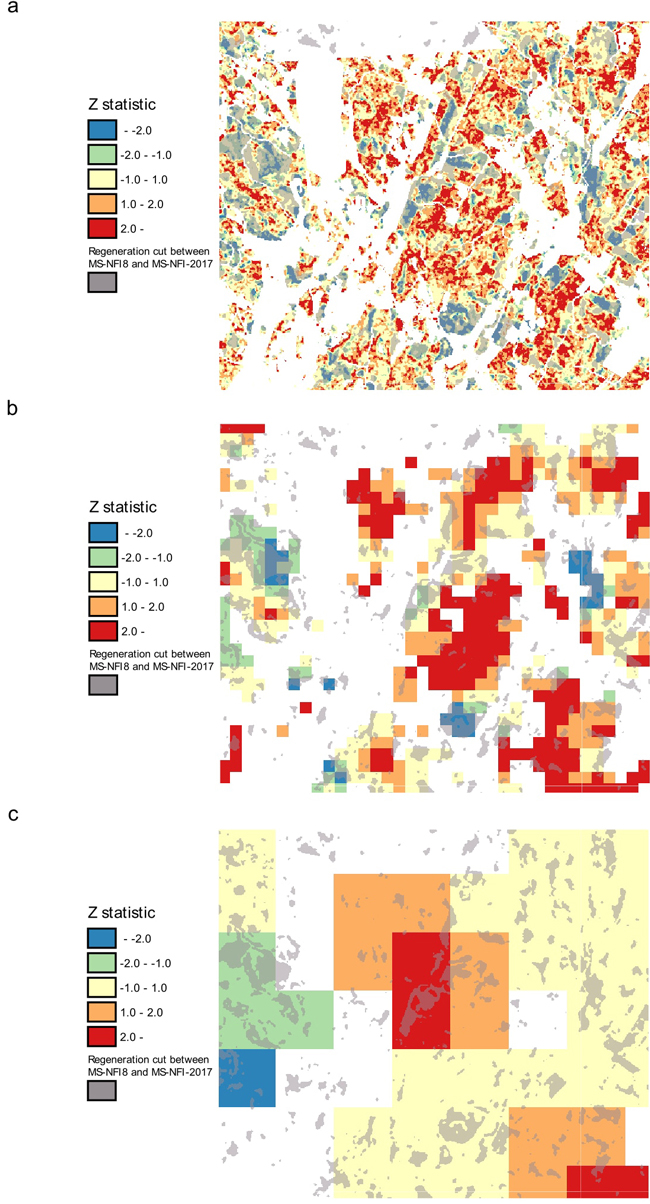
Fig. 3. Contextual Mann-Kendall test to ten multi-source national forest inventory (MS-NFI) mean volume thematic maps, dated 1994–2017, for a subset of Häme test area. The Z statistic for 16 × 16 m2 units (a), 240 × 240 m2 units (b), and 1200 × 1200 m2 units (c). Threshold classification of regeneration cutting areas is shown using the difference between mean volume estimates of growing stock in MS-NFI-8 and MS-NFI-2017 in grey.
At the Häme study site, the trend is positive (Z statistic) in the majority of the 1200 × 1200 m2 units. In the southeast, areas with negative or no trend can be detected (Figs. 4a,b), which can be explained partly by a high proportion of regeneration cuttings visually detected from the regeneration cutting mask. In this area only few units were found with significant (pmulti < 0.05) values. The proportion of non-FRYL masks is relatively high in this area, but that should not affect the sign of the trend in the mean volume map. Changing the unit size to 12 000 × 12 000 m2 retained the geographical patterns of the significant trend and signs of the standardized Z statistic (Figs. 4c,d). However, the total area covered by significant units (pmulti < 0.05) was larger (cf. Table 3). The trend for the mean volume was even more positive and significant in the Kainuu study site (Figs. 4e,f), cf. Table 3. An area deviating from the general trend is pinpointed in Fig. 4e. This area is a large peatland complex containing large open bogs and fens that are difficult to predict in the MS-NFI when using spectral values only.
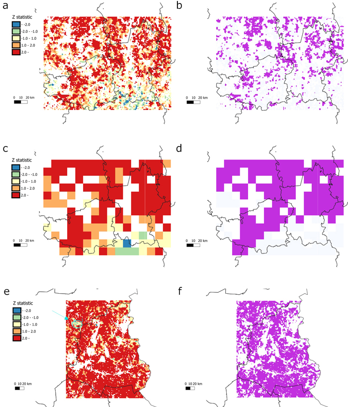
Fig. 4. Contextual Mann-Kendall (CMK) test to ten multi-source national forest inventory (MS-NFI) mean volume thematic maps 1994–2017 at the Häme study site. 1200 × 1200 m2 units and the Z statistic (a), areas with significant trend (pmulti < 0.05) (b), 12 000 × 12 000 m2 units and the Z statistic (c), pmulti < 0.05 (d). CMK test to 9 MS-NFI mean volume thematic maps 1992–2017 at the Kainuu study site. 1200 m units and the Z statistic and a subarea marked (e), pmulti < 0.05 (f). Digital map data: contains data from the National Land Survey of Finland municipal division 1:4.5 M 01/2018. View larger in new window/tab.
4 Discussion
The CMK test showed areas of significant trend (p < 0.05) in a time series of two decades for all the MS-NFI thematic maps analysed at various unit sizes, starting from 16 × 16 m2 pixels. However, multiple testing correction was applied to p-values to guarantee reliable inference from the CMK test, which decreased the number of units with detectable significant trend. The largest proportion of pixels with significant trend (pmulti < 0.05) was found for the mean volume of growing stock. For other variables, significant trends were mostly found for the largest unit size only, 12 000 × 12 000 m2. This unit size represents a small municipality in southern Finland and part of a northern Finland municipality. The sign of the trends was in accordance with the changes in large area estimates from the NFI field data. The employed methods enabled geographical location monitoring for significant changes and trends over time. The declining trends correlated with the predicted areas of regeneration cutting within the time period of the MS-NFIs, particularly for units measuring 240 × 240 m2 and smaller.
In general, the proportion of significant p-values increased with unit size (Tables 2 and 3). However, there is decrease in the proportion at the 1200 × 1200 m2 size units before increasing again at the 12 000 × 12 000 m2 units for some variables: the mean volume in the Häme study site and for the mean volume of spruce on both sites (Table 2). After the multiple testing correction for the p-values (which result we consider more reliable) this phenomenon was seen only for mean volume in Häme study site. We can expect an overall increasing trend for the volume of growing stock based on the NFI time series. On yearly basis, cuttings occur on approximately 3% of forest stands, of which one-third are regeneration cuttings (0.8%) with almost total removal of the growing stock (Finnish Forest Research Institute 2014). If a pixel belongs to a cutting area during the period of the constructed time series, there will be a sudden change in the trend, making it less probable to detect a monotonic trend. The 240 × 240 m2 units cover an area of 5.76 ha and could contain a stand – given an average 1.2 ha stand in southern Finland and a larger stand size in northern Finland – or a group of stands where a cutting has been carried out within the period. It would still affect largely the observed trend. Within the 1200 × 1200 m2 size, there may be several cutting areas and over a period of 23 years (the Häme study area), almost 20% of the stands would be treated with regeneration cutting and nearly 70% would be treated with some type of felling. If the cuttings were located randomly, a positive trend would be expected for the mean volume and even more predominantly for the largest units of 12 000 × 12 000 m2. It is not clear why in some cases the 1200 × 1200 m2 size units have the smallest proportion of significant p-values (Tables 2 and 3). One or more forest estates may be located within this unit size and the drain and volume increment may vary significantly between the estates. Yet the size of the unit is too small to follow the (often positive) large area trend.
The multiple testing correction applied became stronger as the number of tests increased (i.e., the unit size decreased). The number of tests repeated at the Häme study site were 187 799, 11 422 and 138, for the 240 × 240 m2, 1200 × 1200 m2 and 12 000 × 12 000 m2 units, respectively. However, the FDR adjustment of the p-values was a less conservative adjustment among available methods and the probability of finding false positives was not linearly related to the number of tests varying by unit size and given above. Nevertheless, the proportion of the significant p-values decreased 0–20 percentage units for the mean volume of growing stock and the more the smaller the unit size. At the Kainuu study site, the decrease was smaller. For the other variables, the number of units with pmulti < 0.05 went to zero in many cases for the units smaller than 12 000 × 12 000 m2.
The sign of the trends detected in the forest maps were verified at the regional level against the changes in the field data-based estimates. The increasing trend in the mean volume of growing stock agrees with the NFI field inventory statistics, which display increase in the mean volume between 1990’s and 2010’s. The growing stock on forest and poorly productive forest land has increased from the 1890 million m3 in NFI8 (1986–1994) (Tomppo et al. 2001) to 2473 million m3 in NFI12 (2013–2017) (Luke’s Statistics database 2019). Particularly, the increase at the Kainuu site in the volume of growing stock has been large, such as the Kainuu region (number 18 in Fig. 1), where the drain has been only approximately 60% of the volume increment of the growing stock since 2000 (Korhonen et al. 2015b). The mean volume of growing stock for forest and poorly productive forest at the Häme-Uusimaa Public Service Units of the Finnish Forest Centre (covering regions 5 and 7 and northern parts of region 1, see Fig. 1) were 154.4 and 160.2 m3 ha–1 in the NFI9 (1998–1999) and NFI11 (2009–2013), respectively. Those mean volumes at the Kainuu Public Service Unit, which is approximately identical to region 18 (Fig. 1) were 63.9 and 91.2 m3 ha–1 in the NFI8 (1990, 1992) and NFI11 (2009–2013), respectively. Consequently, the proportion of units with significant trend were higher at the Kainuu study site.
The decreasing trend of the mean volume of spruce discovered at the Häme study site agrees with the decrease in the field plot based total growing stock of spruce from 79.1 million m3 to 71.7 million m3 between NFI9 (1998–1999) and NFI11 (2009–2013) at the Häme-Uusimaa Public Service Unit (Korhonen et al. 2000, 2015a). For the stand age, the trend was negative for the 12 000 × 12 000 m2 units, which is in agreement with the decrease in the mean stand age on forest land (national definition) from 56 years to 50 years between NFI9 (1998–1999) and NFI11 (2009–2013) at the Häme-Uusimaa Public Service Unit (Korhonen et al. 2000, 2017). At the Kainuu Public Service Unit, the mean stand age of forest land decreased only slightly, from 62 to 60 years, between NFI9 (2001) and NFI11 (2009–2013) and no trend was detected (pmulti < 0.05); (Tomppo et al. 2003; Korhonen et al. 2015b).
At smaller scale, where the various sizes of units are used, we rely on the CMK test. A set of simulations were used to validate the CMK tests before their application in this study. The CMK test was applied to a purely simulated set of spatial time-series data with combinations of noise, autoregressive model AR(1) and spatially correlated trends. In the course of the simulation study we confirmed the expected multiple testing issue, and after comparing several techniques (such as Bonferroni’s or Holm’s method) for correcting for it, decided on the FDR approach. Based on the simulation trial we could confidently proceed to the data analysis, as the CMK detected trends and the multiple testing correction sharply reduced the false positive rate without being too conservative. The simulations also informed that the prewhitening step is beneficial only in case of strong autocorrelation.
The MS-NFI time-series covered 23 and 25 years containing 10 and 9 observations at different time points in Häme and Kainuu study sites, respectively. The time span in this study is long and significant changes (mainly cuttings) could be expected also at shorter time interval in the Boreal forests. However, the annual increment of growing stock in Finland is rather low, 4% on average on the forest and poorly productive forest land (national definition) (Luke’s Statistics database 2019). Czerwinski et al. (2014) tested the sensitivity of trend analysis to the time interval between images in their 20-year time-series set of Landsat data. The 4–5 year interval produced similar change results as 1–3 year interval of the time series. In our case, as the suggested number of observations is n ≥ 8 for the MK test we did not test for shorter time-series or longer time intervals. The intervals were longer between the first three MS-NFIs which was not taken into account formally in the calculations of the CMK test statistic. However, we assume that this will not largely distort the results.
At the pixel level, the root mean squared error of the MS-NFI predictions can be large, with 50–80% applying leave-one-out cross-validation (Tokola and Heikkilä 1997; Katila and Tomppo 2002). The variation explained by the k-NN prediction of the mean volumes by tree species groups is usually lower than that of the mean volume of growing stock (Katila and Tomppo 2002). There are several error sources in the MS-NFI, including location errors, atmospheric effects and limitations in radiometric resolutions and imaging techniques of the satellite sensors (Tomppo et al. 2008). However, the seasonal and atmospherical effects (Zhu 2017) typical in multitemporal analysis are expected to be avoided in part because the best quality images were selected from the growing season and a careful manual cloud detection was carried out in the MS-NFI (Mäkisara et al. 2019). The MS-NFI prediction errors increase the variance in the time series of the forest variables between different time point MS-NFIs. The standard errors decrease as the pixel-level predictions are aggregated and the area size increases (Katila 2006). Trends become more consistent as unit sizes increase (Fig. 2). This could be another reason, in addition to the distribution of the cutting areas, for the larger amount of significant test values at the largest unit size. There may be also systematic errors in the MS-NFI estimates between large regions, partly due to changes in the estimation methods. For example, MS-NFI-2007 seems to have smaller mean volumes in Table 1 and on longitudinal plots of a sample for single units (Fig. 2). Nevertheless, the CMK test managed to detect significant trends despite deviations of single observations in the time series.
It is known that peatlands may experience variation between earlier MS-NFIs and the latest ones on the level of mean volume predictions on open bogs and fens causing unwanted trends. These are often nearly treeless areas but have a large spectral variation in the satellite images (Tomppo et al. 2008). Therefore, the results for the open bogs and fens should be checked separately or masked to null as the expectation in the growing stock is no change.
Parts of non-FRYL masks were included in larger-than-pixel units. The non-FRYL mask pixels were set to zero in the calculation of the unit values. This decreased the mean values and the unit variation compared to the variation in original values on the FRYL mask. Hence, deforestation and afforestation also affected the unit values, but CMK tests only the sign of the trend and including non-FRYL pixels does not change the trend in the mean values of the units.
The map units used did not follow the forest stand delineation typical in the silvicultural practice of Finland. A delineation based on auxiliary data or segmentation methods could be used to form the units following stand boundaries to search for trends (Descle et al. 2006). This would probably decrease the variation within units. However, the rectification errors in the MS-NFI maps are only minor compared to the unit sizes tested (240 × 240 m2 and larger) and real trends are assumed to be detected despite forest stands being split between the rectangular units used in this study.
Neeti and Eastman (2011) applied prewhitening (Wang and Swail 2001) to remove serial autocorrelation from time series data. However, there have been objections to the use of prewhitening (Yue and Wang 2002). We observed in our simulation study that prewhitening increased the variance of the test statistic, reducing the power of the test. In addition, an exploratory analysis of a set of randomly selected pixels revealed no significant autocorrelation, so this study did not use prewhitening.
The results support the hypothesis that significant trends can be detected with the trend analysis from the scale of forest estates onwards. Significant trends can be detected from k-NN based forest maps, optical area satellite images covering sufficient number of time points from a regular time interval (in this case, a time span of two decades) and relatively consistent materials and methodology. The CMK test proved applicable for the task, but a more demanding task is to estimate the magnitude of change in measurable units, such as mean volumes or biomass.
The detected significant trends can be used as indicators of sustainability of forest management at various scales, specifically in smaller scales than possible with NFI field sample data only. For instance, in the mean volume a positive trend indicates that growth is higher than drain, which is considered as one indicator of sustainable use of forest resources. A positive trend in the proportion of broadleaved trees would indicate increasing proportion of mixed forests, which is one indicator for sustainable forest management. Thus, trend analysis can provide indicators for assessing sustainability with regards to such parameters that can be assessed with remote sensing. A significant positive trend is a strong indicator of the sustainability, and a lack of negative trend a weaker indicator of sustainability. Both interpretations support the assumption of sustainability at the study sites in the two largest scales with respect to the considered indicators. The two smaller scales are more suitable to assessment of abrupt changes, as harvests dominate the trend.
It needs to be acknowledged, however, that sustainability is hard – maybe impossible – to define in such a way that would account for all necessary aspects. Therefore, trend analysis like this can only provide indicative information supporting or not supporting sustainability of the forest use from certain perspectives. Yet, such information can be useful e.g. for local forest administration or policy processes.
Significant trends could be observed in the two largest scales, of which the 1200 × 1200 m2 scale was assumed to represent a large forest estate. Yet, it cannot be assumed that sustainability would be possible or even desirable in all such pixels. Thus, when the scale becomes smaller, the proportion of positive and negative trends in a larger area would be a better indicator of sustainability than the observed trend in each pixel. While for detecting the trends as such both the larger scales of this study seem appropriate, the role of scale in sustainability considerations requires more studies.
Acknowledgements
We thank Lic. Tech. Kai Mäkisara for advice on image processing matters. This work was supported by the “Open Geospatial Information Infrastructure for Research - oGIIR” project, Academy of Finland.
References
Benjamini Y., Yekutieli D. (2001). The control of the false discovery rate in multiple testing under dependency. The Annals of Statistics 29(4): 1165–1188. https://doi.org/10.1214/aos/1013699998.
Coops N.C., Shang C., Wulder M.A., White J.C., Hermosilla T. (2020). Change in forest condition: Characterizing non-stand replacing disturbances using time series satellite imagery. Forest Ecology and Management 474: 118–370. https://doi.org/10.1016/j.foreco.2020.118370.
Corona P., Chirici G., McRoberts R.E., Winter S., Barbati A. (2011). Contribution of large-scale forest inventories to biodiversity assessment and monitoring. Forest Ecology and Management 262(11): 2061–2069. https://doi.org/10.1016/j.foreco.2011.08.044.
Czerwinski C.J., King D.J., Mitchell S.W. (2014). Mapping forest growth and decline in a temperate mixed forest using temporal trend analysis of Landsat imagery, 1987–2010. Remote Sensing of Environment 141: 188–200. https://doi.org/10.1016/j.rse.2013.11.006.
Czúcz B., Condé S. (2018). Ecosystem type fact sheet on forests. Technical Report 12g/2018, European Environment Agency. https://www.eionet.europa.eu/etcs/etc-bd/products/etc-bd-reports/etc-bd-report-12-2018-fact-sheets-on-ecosystem-condition/@@download/file/ETCBD_Technical_report_12-2018.zip.
Desclée B., Bogaert P., Defourny P. (2006). Forest change detection by statistical object-based method. Remote Sensing of Environment 102(1–2): 1–11. https://doi.org/10.1016/j.rse.2006.01.013.
Finnish Forest Research Institute (2014). Finnish statistical yearbook of forestry 2014. Finnish Forest Research Institute, Vantaa, Finland. http://urn.fi/URN:ISBN:978-951-40-2506-8.
Forest resource maps and municipal statistics (2020). Forest resource maps and municipal statistics. Natural Resources Institute (Luke), Finland. https://www.luke.fi/en/natural-resources/forest/forest-resources-and-forest-planning/forest-resource-maps-and-municipal-statistics/. [Cited 8 Jan 2020].
Gómez C., White J.C., Wulder M.A. (2011). Characterizing the state and processes of change in a dynamic forest environment using hierarchical spatio-temporal segmentation. Remote Sensing of Environment 115(7): 1665–1679. https://doi.org/10.1016/j.rse.2011.02.025.
Goovaerts P. (2010). How do multiple testing correction and spatial autocorrelation affect areal boundary analysis? Spatial and Spatio-temporal Epidemiology 1(4): 219 – 229. https://doi.org/10.1016/j.sste.2010.09.004.
Haakana H. (2017). Multi-source forest inventory data for forest production and utilization analyses at different levels. Dissertationes Forestales 243. 63 p. https://doi.org/10.14214/df.243.
Katila M. (2006). Empirical errors of small area estimates from the multisource national forest inventory in Eastern Finland. Silva Fennica 40(4): 729–742. https://doi.org/10.14214/sf.324.
Katila M., Tomppo E. (2002). Stratification by ancillary data in multisource forest inventories employing k-nearest neighbour estimation. Canadian Journal of Forest Research 32(9): 1548–1561. https://doi.org/10.1139/x02-047.
Kendall M.G. (1975). Rank correlation methods. Charles Griffin, London.
Kerr J.T., Ostrovsky M. (2003). From space to species: ecological applications for remote sensing. Trends in Ecology and Evolution 18(6): 299–305. https://doi.org/10.1016/S0169-5347(03)00071-5.
Korhonen K.T., Tomppo E., Henttonen H., Ihalainen A., Tonteri T. (2000). Hämeen-Uudenmaan metsäkeskuksen alueen metsävarat 1965–1999. [Forest resources of Häme-Uusimaa forestry centre 1965–1999]. Folia Forestalia 3B/2000: 489–566. [In Finnish]. http://urn.fi/URN:NBN:fi-fe2016111829363.
Korhonen K.T., Ihalainen A., Packalen T., Salminen O., Hirvelä H., Härkönen K. (2015a). Hämeen metsävarat ja hakkuumahdollisuudet. [Forest resources and felling possibilities of Häme]. 26 p. Natural Resources Institute (Luke), Finland. [In Finnish]. http://urn.fi/URN:NBN:fi-fe201603218855.
Korhonen K.T., Ihalainen A., Packalen T., Salminen O., Hirvelä H., Härkönen K. (2015b). Kainuun metsävarat ja hakkuumahdollisuudet. [Forest resources and felling possibilities of Kainuu]. 26 p. Natural Resources Institute (Luke), Finland. [In Finnish]. http://urn.fi/URN:NBN:fi-fe201603218856.
Korhonen K.T., Ihalainen A., Ahola A., Heikkinen J., Henttonen H.M., Hotanen J.-P., Nevalainen S., Pitkänen J., Strandström M., Viiri H. (2017). Suomen metsät 2009–2013 ja niiden kehitys 1921–2013. [The forests of Finland 2009–2013 and their development in 1921–2013]. Natural resources and bioeconomy studies 59/2017. Natural Resources Institute Finland (Luke). [In Finnish]. http://urn.fi/URN:ISBN:978-952-326-467-0.
Luke’s Statistics database (2019). Luke’s statistics database. Natural Resources Institute (Luke), Finland. https://stat.luke.fi/en/uusi-etusivu. [Cited 11 Oct 2019].
Mäkisara K., Heikkinen J., Heiler I., Henttonen H., Katila M., Pitkänen J., Tomppo E. (2001). Valtakunnan metsien inventoinnin (VMI) ajantasaistus kaukokartoitusaineiston avulla. Tutkimushankkeen loppuraportti. [Updating of the Finnish national forest inventory using remote sensing data. Final report.] Finnish Forest Research Institute (Metla). [In Finnish].
Mäkisara K., Katila M., Peräsaari J., Tomppo E. (2016). The multi-source national forest inventory of Finland – methods and results 2013. Natural resources and bioeconomy studies 10/2016. Natural Resources Institute Finland (Luke). http://urn.fi/URN:ISBN:978-952-326-186-0.
Mäkisara K., Katila M., Peräsaari J. (2019). The multi-source national forest inventory of Finland – methods and results 2015. Natural resources and bioeconomy studies 8/2019. Natural Resources Institute Finland (Luke). http://urn.fi/URN:ISBN:978-952-326-711-4.
Mann H.B. (1945). Nonparametric tests against trend. Econometrica 13(3): 245–259. https://doi.org/10.2307/1907187.
McRoberts R.E., Cohen W.B., Næsset E., Stehman S.V., Tomppo E.O. (2010). Using remotely sensed data to construct and assess forest attribute maps and related spatial products. Scandinavian Journal of Forest Research 25(4): 340–367. https://doi.org/10.1080/02827581.2010.497496.
Neeti N., Eastman J.R. (2011). A contextual Mann-Kendall approach for the assessment of trend significance in image time series. Transactions in GIS 15(5): 599–611. https://doi.org/10.1111/j.1467-9671.2011.01280.x.
Open Geospatial Information Infrastructure for Research (2020). R-package: contextual Mann-Kendall trend test for rasterStacks. https://github.com/geoporttishare/ConMK. [Cited 27 Mar 2020].
Parviainen J., Västilä S. (2011). Suomen metsät 2011 - kestävän metsätalouden kriteereihin ja indikaattoreihin perustuen. [The forests of Finland 2011 - based on criteria and indicators of sustainable forest management]. Maa- ja metsätalousministeriön julkaisuja 5/2011. Maa- ja metsätalousministeriö, Helsinki, Finland. [In Finnish]. http://urn.fi/URN:ISBN:978-952-453-665-3.
Pitkänen T., Sirro L., Häme L., Häme T., Törmä M., Kangas A. (2020). Errors related to the automatized satellite-based change detection of boreal forests in Finland. International Journal of Applied Earth Observations and Geoinformation 86 article 102011. 10 p. https://doi.org/10.1016/j.jag.2019.102011.
R Core Team (2020). R: a language and environment for statistical computing. R Foundation for Statistical Computing, Vienna, Austria. http://www.R-project.org/. [Cited 27 Mar 2020].
Rocchini D., Marcantonio M., Re D.D., Chirici G., Galluzzi M., Lenoir J., Ricotta C., Torresani M., Ziv G. (2019). Time-lapsing biodiversity: an open source method for measuring diversity changes by remote sensing. Remote Sensing of Environment 231 article 111192. https://doi.org/10.1016/j.rse.2019.05.011.
Saarinen N., White J., Wulder M., Kangas A., Tuominen S., Kankare V., Holopainen M., Hyyppä J., Vastaranta M. (2018). Landsat archive holdings for Finland: opportunities for forest monitoring. Silva Fennica 52(3) article 9986. 11 p. https://doi.org/10.14214/sf.9986.
Tokola T., Heikkilä J. (1997). Improving satellite image based forest inventory by using a priori site quality information. Silva Fennica 31(1): 67–78. https://doi.org/10.14214/sf.a8511.
Tomppo E. (1990). Satellite image-based national forest inventory of Finland. The Photogrammetric Journal of Finland 12: 115–120.
Tomppo E., Halme M. (2004). Using coarse scale forest variables as ancillary information and weighting of variables in k-nn estimation: a genetic algorithm approach. Remote Sensing of Environment 92(1): 1–20. https://doi.org/10.1016/j.rse.2004.04.003.
Tomppo E., Katila M. (1991). Satellite image-based national forest inventory of Finland. In: Proceedings of the International Geoscience and Remote Sensing Symposium, IGARSS’91. IEEE. p. 1141–1144.
Tomppo E., Katila M., Moilanen J., Mäkelä H., Peräsaari J. (1998). Kunnittaiset metsävaratiedot 1990–94. [Forest resources by municipalities 1990–1994]. Metsätieteen aikakauskirja 4B/1998: 619–839. [In Finnish]. https://doi.org/10.14214/ma.6453.
Tomppo E., Henttonen H., Tuomainen T. (2001). Valtakunnan metsien 8. inventoinnin menetelmä ja tulokset metsäkeskuksittain Pohjois-Suomessa 1992–94 sekä tulokset Etelä-Suomessa 1986–92 ja koko maassa 1986–94. [The methods of the 8th national forest inventory and the results by forestry centres in North Finland and in whole country]. Metsätieteen aikakauskirja 1B/2001: 99–248. [In Finnish]. https://doi.org/10.14214/ma.6434.
Tomppo E., Henttonen H., Ihalainen A., Tonteri T. (2003). Kainuun metsäkeskuksen alueen metsävarat 1969–2001. [Forest resources of Kainuu forestry centre 1969–2001]. Folia Forestalia 2B/2003: 169–256. [In Finnish]. https://doi.org/10.14214/ma.5787.
Tomppo E., Haakana M., Katila M., Peräsaari J. (2008). Multi-Source National Forest Inventory. Methods and applications. Managing Forest Ecosystems 18. Springer, Dodrecht, The Netherlands. 374 p.
Tomppo E., Haakana M., Katila M., Mäkisara K., Peräsaari J. (2009). The Multi-source National Forest Inventory of Finland – methods and results 2005. Working Papers of the Finnish Forest Research Institute 111. 277 p. http://urn.fi/URN:ISBN:978-951-40-2151-0.
Tomppo E., Heikkinen J., Henttonen H., Ihalainen A., Katila M., Mäkelä H., Tuomainen T., Vainikainen N. (2011). Designing and conducting a forest inventory-case: 9th National Forest Inventory of Finland. Springer Verlag. https://doi.org/10.1007/978-94-007-1652-0.
Tomppo E., Katila M., Mäkisara K., Peräsaari J. (2012). The multi-source national forest inventory of Finland – methods and results 2007. Working Papers of the Finnish Forest Research Institute 227. 233 p. http://urn.fi/URN:ISBN:978-951-40-2357-6.
Tomppo E., Katila M., Mäkisara K., Peräsaari J. (2013). The multi-source national forest inventory of Finland – methods and results 2009. Working Papers of the Finnish Forest Research Institute 273. 216 p. http://urn.fi/URN:ISBN:978-951-40-2428-3.
Tomppo E., Katila M., Mäkisara K., Peräsaari J. (2014). The multi-source national forest inventory of Finland – methods and results 2011. Working Papers of the Finnish Forest Research Institute 319. 224 p. http://urn.fi/URN:ISBN:978-951-40-2516-7.
Vauhkonen J., Ruotsalainen R. (2017). Assessing the provisioning potential of ecosystem services in a Scandinavian boreal forest: suitability and tradeoff analyses on grid-based wall-to-wall forest inventory data. Forest Ecology and Management 389: 272–284. https://doi.org/10.1016/j.foreco.2016.12.005.
Wallerman J. (2003). Remote sensing aided spatial prediction of forest stem volume. Ph.D. thesis, Swedish University of Agricultural Sciences, Forest Resorce Management and Geomatics. Acta Universitatis Agriculturae Sueciae. Silvestria 271.
Wang X.L., Swail V.R. (2001). Changes of extreme wave heights in northern hemisphere oceans and related atmospheric circulation regimes. Journal of Climate 14(10): 2204–2221. https://doi.org/10.1175/1520-0442(2001)014%3C2204:COEWHI%3E2.0.CO;2.
White J.C., Wulder M.A., Hobart G.W., Luther J.E., Hermosilla T., Griffiths P., Coops N.C., Hall R.J., Hostert P., Dyk A., Guindon L. (2014). Pixel-based image compositing for large-area dense time series applications and science. Canadian Journal of Remote Sensing 40(3): 192–212. https://doi.org/10.1080/07038992.2014.945827.
Winter S., McRoberts R.E., Bertini R., Bastrup-Birk A., Sanchez C., Chjrici G. (2011) Essential features of forest biodiversity for assessment purposes. In: Chirici G., Winter S., McRoberts R.E. (eds.). National forest inventories: contributions to forest biodiversity assessments. Springer, Berlin and Heidelberg. p. 25–39. https://doi.org/10.1007/978-94-007-0482-4_2.
Wulder M.A., Masek J.G., Cohen W.B., Loveland T.R., Woodcock C.E. (2012). Opening the archive: how free data has enabled the science and monitoring promise of Landsat. Remote Sensing of Environment 122: 2–10. https://doi.org/10.1016/j.rse.2012.01.010.
Yue S., Wang C.Y. (2002). Regional streamflow trend detection with consideration of both temporal and spatial correlation. International Journal of Climatology 22(8): 933–946. https://doi.org/10.1002/joc.781.
Zhu Z. (2017). Change detection using Landsat time series: a review of frequencies, preprocessing, algorithms, and applications. ISPRS Journal of Photogrammetry and Remote Sensing 130: 370–384. https://doi.org/10.1016/j.isprsjprs.2017.06.013.
Total of 53 references.
