Sören Wulff  ,
Cornelia Roberge,
Anna Hedström Ringvall,
Sören Holm,
Göran Ståhl
,
Cornelia Roberge,
Anna Hedström Ringvall,
Sören Holm,
Göran Ståhl
On the possibility to monitor and assess forest damage within large scale monitoring programmes – a simulation study
Wulff S., Roberge C., Ringvall A. H., Holm S., Ståhl G. (2013). On the possibility to monitor and assess forest damage within large scale monitoring programmes – a simulation study. Silva Fennica vol. 47 no. 3 article id 1000. https://doi.org/10.14214/sf.1000
Abstract
There is a growing demand for information on forest health due to fears that climate change may cause new kinds of damage that have not previously been encountered. In many cases, forest damage monitoring is conducted exclusively within sparse large-scale grids of sample plots and it is doubtful whether these are capable of providing relevant information to support mitigation programmes or other actions required to reduce economic losses due to damage outbreaks. In this study, we used simulated sampling to assess the precision of estimators related to forest state and changes in the damage sustained by trees within an area corresponding to the Swedish region Götaland, assuming a sampling design corresponding to that used in the Swedish National Forest Inventory (NFI) under different damage scenarios. Large and uniformly distributed damage outbreaks were well captured by an NFI-type inventory, but scattered damage outbreaks produced estimates with poor precision. As a consequence, we propose that there might be a need to revise current forest damage monitoring programmes to make them more useful for monitoring the kinds of damage that are likely to arise as a consequence of climate change.
Keywords
forest health;
forest inventory;
environmental monitoring and assessment;
forest condition
-
Wulff,
Swedish University of Agricultural Sciences, Department of Forest Resource Management, Skogsmarksgränd, SE-901 83 Umeå, Sweden
E-mail
soren.wulff@slu.se
- Roberge, Swedish University of Agricultural Sciences, Department of Forest Resource Management, Skogsmarksgränd, SE-901 83 Umeå, Sweden E-mail cornelia.roberge@slu.se
- Ringvall, Swedish University of Agricultural Sciences, Department of Forest Resource Management, Skogsmarksgränd, SE-901 83 Umeå, Sweden E-mail anna.ringvall@slu.se
- Holm, Swedish University of Agricultural Sciences, Department of Forest Resource Management, Skogsmarksgränd, SE-901 83 Umeå, Sweden E-mail soren.holm@slu.se
- Ståhl, Swedish University of Agricultural Sciences, Department of Forest Resource Management, Skogsmarksgränd, SE-901 83 Umeå, Sweden E-mail goran.stahl@slu.se
Received 10 July 2012 Accepted 15 February 2013 Published 25 September 2013
Views 181697
Available at https://doi.org/10.14214/sf.1000 | Download PDF

Supplementary Files
1 Introduction
Global climate change presents significant risks to a number of important ecosystems, including those of Scandinavian boreal forests (Dale et al. 2001). Consequently, there is a growing demand for reliable and up-to-date information on forest health and for effective methods of monitoring damage to trees and forests as a whole. This has been accompanied by changes in the nature of the information required to evaluate forest health. Notably, the crown condition assessments introduced in the 1980s (Lorenz 1995) in response to the threats posed by air pollution need to be complemented by assessments of specific damage types and their causes as well as populations of potential damaging agents and early signs of damage outbreaks (Lovett et al. 2007). Information of this sort can be used to inform and adapt forest management practices in order to avoid major risks or to draw up specific mitigation programmes to minimize the impact of damage outbreaks that are in progress (Wulff et al. 2012).
However, designing monitoring programmes that meet these information requirements is far from trivial. As pointed out by Ferretti (2009) and Wulff (2004), one important issue to consider is that the selected methods must deliver results that are consistent over time; were this not the case, it would be impossible to correctly interpret any trends that were identified. In general, the best way to achieve this goal is to use probability sampling methods, since they provide unbiased estimators whose precision can be estimated (Schreuder et al. 2001; Russek-Cohen and Christman 2004). Permanent sampling units are preferred for detecting changes in the state of the targeted forest (McRoberts et al. 2010b). Many large-scale national and transnational forest damage monitoring programmes have been established, such as the International Cooperation Programme ICP Forests network, which acts under the aegis of the Convention on long-range transboundary air pollution (Lorenz 1995). Monitoring technologies and methods are developed on an ongoing basis within the ICP forests program. As part of the European FutMon programme (FutMon 2011) steps have been taken to establish a new large-scale probability sampling monitoring grid in the form of a so-called ICP Forests level 1 grid that would be connected to on-going national forest inventories (NFIs) (Tomppo et al. 2010). As a result of this, many European countries nowadays assess forest health and forest damage in a way that is either fully integrated into their NFIs or as part of a grid that is at least partially co-located with the NFI. For example, Sweden has chosen to fully integrate its national damage assessments into its NFI. In parallel with these European developments, the US Forest Health Monitoring program (USDA 2011) has merged its operations and data into the NFI sampling grid (Shaw 2008).
A common feature of most NFIs is that they are based on a sparse systematic probability sample of field plots, which are often laid out in clusters (Lawrence et al. 2010; McRoberts et al. 2010b). Many NFIs are at least partially based on permanent plots that are revisited at specific intervals, typically of five to ten years (Lawrence et al. 2010; McRoberts et al. 2010b). In most cases, the total sample is split into so-called panels, each of which contains the subsets of the sample that will be visited within a given year. Each panel contains plots spanning the entire study area (Bechtold and Pattersson 2005). By performing ongoing inventories with long periods between site revisits, one can obtain a very large total sample size. However, the resulting estimates typically need to be presented in the form of moving averages based on data from several years in order to be reliable.
Another common feature of NFIs is that they are generally dimensioned to provide estimates with acceptable precision at the national level, or at the sub-national level when dealing with large regions; their primary focus is usually on growing stock and related estimates, although many NFIs have acquired multiple purposes over the years (McRoberts et al. 2010b).
While Nordic forests could potentially suffer numerous different kinds of damage, the most severe problems have a few specific causes. One of the most severe disturbances that affect Nordic forests is decay, which is a widespread problem with major economic implications (Oliva et al. 2010). Another is grazing by ungulates, which can cause substantial destruction in young forests (Apollonio et al. 2010). A third is damage from extreme weather events such as huge storms, which is often followed by serious insect outbreaks. The winter storms in 2005 and 2007 were exceptionally severe, felling an estimated 75 million m3sk (total trunk volume over bark above stump) and 12 million m3sk in Sweden alone (Jonsson 2008). The subsequent insect outbreaks in 2006 –2010 are estimated to have destroyed ca. 3 million m3sk (Långström et al. 2009). Further, epidemic outbreaks of the fungus Gremmeniella have affected several hundred thousand ha of pine forest (Nevalainen et al. 2010).
Trees that have sustained different types of damage are normally relatively sparsely distributed and scattered across the forest landscape. Further, damage often occurs in aggregated patterns. It has previously been shown by Nevalainen (1999), Wulff et al. (2006), and Nevalainen et al. (2010) that NFI-type monitoring programmes have the potential to provide reliable information in the event of large-scale damage. However, Edgar and Burk (2006) concluded that extensive forest health monitoring networks are most likely to be useful for monitoring very large, affecting more than several hundred thousand hectares, damage outbreaks and cannot reliably capture smaller outbreaks that may nevertheless be economically significant. Due to the increasing demands for damage information and the current integration of health and damage monitoring into NFIs or NFI-type inventories, it would be useful to determine the ability of such programmes to quantify the effects of different varieties of damage outbreaks with sufficient precision to yield estimates that can be used in decision making.
The capabilities of forest damage monitoring programmes have been evaluated in various empirical studies (Nevalainen 1999; Wulff et al. 2006 and Nevalainen et al. 2010) but there remains a need for more extensive evaluations with a broader scope. A number of different sampling strategies for use in damage assessment have been developed (Ferretti 1997; Alexander et al. 2005). The sampling designs used in NFI-type inventories must be effective and perform well in a wide range of applications, and so it is important to evaluate a design’s performance. Simulation is a useful tool for evaluating the performance of sampling designs (Legendre et al. 2002; Edgar and Burk 2006). For example, Baffetta et al. (2011) used Monte-Carlo techniques to simulate sampling in artificial populations and thereby evaluate the potential for reliably assessing the properties of trees outside the targeted forests within a NFI-type inventory. Simulated sampling in artificial populations can be used to study the performance of specific sampling designs in many different outbreak scenarios and thus makes it possible to identify factors that affect the precision of the resulting estimates, such as outbreak intensity and the aggregation of damage.
The aim of this study was to investigate the advantages and disadvantages of using NFI-type designs to monitor and assess different kinds of forest damage outbreaks at the sub-national level. Specifically, the aim was to examine the potential to detect and quantify forest damage in simulated cases that represent a range of damage types and intensities. Evaluations were performed based on simulated sampling of simulated populations and focused on the precision of state and increment estimators of the number of damaged trees ha–1 in a large study area, corresponding to the Götaland region of Sweden. We considered a general, large-scale, sampling design, and related its sampling intensity to that of the Swedish NFI (Axelsson et al. 2010).
2 Methods
2.1 Study area, variable of interest and sampling design
The study was performed using a simulated region of exclusively forested land with an area of 50 000 km2. This is approximately the area of productive forest land in Sweden’s southernmost region, Götaland (Forestry statistics 2010 … 2010), and was selected because there is often a need to obtain precise estimates based on NFI data for forested areas of around this size. In practical situations where one is only interested in the properties of forested land, data for plots containing other types of land are often disregarded, and estimates for forest land are produced using ratio estimators (e.g., Zarnoch and Bechtold 2000). To avoid introducing non-forest land types into our simulations, we included only forest land in our simulated region and considered a number of plots that is roughly equal to the number of NFI plots lying on forested land in Götaland rather than the total number of NFI plots within the region, some of which lie on other types of land. This is equivalent to the procedure that would be adopted in a real-world situation where the distribution of forest land within the region of interest was known in advance, making it possible to select a sample of the studied size from within the forested area in a controlled manner (Särndal et al. 1992, p. 393).
The severity of the forest damage sustained in a given incident can be determined by considering quantities such as the total area affected by (for example) a pest or disease, or the proportion of trees affected (Wulff et al. 2006). In this work, we focused on the mean number of affected trees per hectare, i.e. the density of damaged trees rather than the proportion of trees affected. This made it possible to simulate damaged trees as point processes. We considered estimators of both the increase in the number of damaged trees ha–1 between two time points and the current number of damaged trees ha–1 at a given time point. When evaluating outbreaks, it is often desirable to examine both a general estimator of the outbreak’s extent and a separate estimator of the number or proportion of trees showing signs of recent damage (Wulff et al. 2006). In this study, the estimator of the increase in the number of damaged trees ha–1 between two adjacent time points is equivalent to an estimator of the number of trees per hectare that show signs of recent damage.
As mentioned previously, many NFIs, including the Swedish NFI, utilize a systematic sampling design. Due to the large size of the study area considered in this work and the resulting large number of trees exhibiting damage symptoms, it would have been very computationally demanding to simulate a systematic layout of sampling locations covering the entire study area. Instead, we divided the study area into 500 equally sized non-overlapping squares with dimensions of 10 × 10 km (see Fig. 1). A single sampling location within each of these squares was selected independently. This type of design is used in the US’ national forest inventory (the FIA), among others (McRoberts et al. 2010a), albeit with tessellation into hexagons rather than squares. The lengths of the squares’ sides were chosen to correspond to the distance between sampling locations given a systematic design with a certain number of sampling locations. Consequently, the area of each square corresponds to the area that would contain exactly one sampling location in a systematic design. Comparisons of the performance of ordinary systematic designs and the unaligned systematic design used in our study have been presented by Cochran (1977, p. 210) and references therein, and by Dunn and Harrison (1993).
A cluster of eight fixed-area plots was selected in each sampling location. All of the plots were permanent, i.e. measurements were taken in the same places at all time points considered. The sampling design thus featured 500 clusters, each of which contained eight fixed-area plots. This is similar to the design adopted by the Swedish NFI in Götaland, which in 2009 featured 250 permanent clusters of eight circular plots; this means that over a five-year period, measurements would be conducted in 1250 plot clusters. Around 50% of the plots in this region lie on productive forest land (Jonas Fridman, Head of the Swedish NFI, pers. comm. in 2011). After a sudden damage outbreak, it might be of interest to estimate the extent of the outbreak using only data from the current year’s panel. Given a five year period between revisits to permanent plots, the yearly inventory would consist of n = 100 plot clusters.
2.2 Simulation of damaged trees
Simulations of tree damage were performed for two main event scenarios that were both based on real-world damage events. The two scenarios were:
- Sparsely and uniformly distributed damage. The damage covers the entire area and is dispersed slowly with low aggregation. This scenario is based on the outbreak of resin top disease, which is estimated to affect 3.6 trees ha–1 in middle aged and older pine forests in Götaland (Swedish NFI).
- Local or regional outbreaks with aggregated centres. In this scenario, the damage is typically present at a low level, but can rapidly increase under favourable conditions, such as optimal weather conditions. The dispersion of damage is typically rapid and aggregated. This scenario is based on the Gremmeniella epidemic of 2001–2003, which is estimated to have affected 61 trees ha–1 in middle aged and older pine forests in Götaland (Swedish NFI).
Many damage events only affect members of a single tree species of a given age and so evidence of damage will appear in patches at the landscape level. This was accounted for by using study areas that have a mixture of empty squares that contain no damaged trees, and squares containing damaged trees. For each of the two event scenarios, we considered study areas with varying proportions (P) of squares with damaged trees. The scenarios were set up on a square-by-square basis by first simulating the positions of damaged trees at an initial time point (TP1) and then simulating the increase in the number of damaged trees between TP1 and a subsequent time point, TP2. The total population of damaged trees at TP2 was then determined in terms of the total number of damaged trees at TP1 plus the number of newly damaged trees (Fig. 1). In reality, some trees that had sustained the type of damage being considered would disappear between TP1 and TP2 (due to mortality or logging) or would recover from the damage they had previously sustained. However, we assumed this number to be negligibly small relative to the total number of damaged trees at TP2.
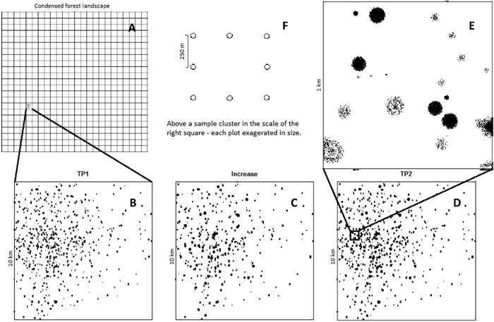
Fig. 1. Example of a simulated population in Scenario 2. The study area contains a total of 500 10×10 km squares. (A) A given proportion of these squares were chosen to contain damaged trees; the rest contained no damaged trees. Subfigures B-D show a single such 10×10 km square, with damaged trees indicated by black spots. Subfigure B shows a square containing 238 tree damage aggregation centres at the initial time point (TP1). Subfigure C shows an increment in which the intensity of all of the aggregation centres is increased, and 38 of them have increased in radius. Subfigure D shows the resulting population of damaged trees at a subsequent time point (TP2).
For each of the two main scenarios, we simulated the density of trees at two levels of intensity (in terms of the number of damaged trees ha–1) within the non-empty squares. In the case of TP1, the two levels were referred to as the sparse and medium intensities; in the case of the increase between TP1 and TP2, the two levels were referred to as the small and the large increase. Four sub-scenarios were thus constructed for each of the two main scenarios, with different increases between TP1 and TP2, and different final states at TP2. To introduce variability in factors such as the number of damaged trees ha–1 in different squares, the parameters of the simulated point processes were specified in terms of minimum and maximum values for some variables, while other variables had fixed values (see Table 1 for Scenario 1 and Table 2 for Scenario 2). The actual value in a specific square was then selected from a uniform distribution between the maximum and minimum values; in the following paragraphs, this selection is referred to as U(min,max).
| Table 1. Parameters for the simulations of damaged trees in Scenario 1, with values set for simulated alternatives of damage level at an initial time point, TP1, and increases to a subsequent time point, TP2. | ||||
| TP1 | Sparse | Medium | ||
| Min no. trees ha–1 | 0.5 | 5 | ||
| Max no. trees ha–1 | 2.5 | 20 | ||
| Increase | Small | Large | Small | Large |
| Min new trees ha–1 | 0.05 | 9 | 0.5 | 38 |
| Max new trees ha–1 | 0.4 | 20 | 2 | 48 |
| Table 2. Parameters for simulations of damaged trees in Scenario 2, with values set for simulated alternatives of damage level at an initial time point, TP1, and increases to a subsequent time point, TP2. | ||||
| TP1 | Sparse | Medium | ||
| Min no aggregation centres square–1 | 200 | 500 | ||
| Max no aggregation centres square–1 | 800 | 1500 | ||
| Min aggregation centres radius (m) | 5 | 5 | ||
| Max aggregation centres radius (m) | 50 | 50 | ||
| Min no trees ha–1 within aggregation centres | 100 | 250 | ||
| Max no trees ha–1 within aggregation centres | 200 | 350 | ||
| Increase | Small | Large | Small | Large |
| Prob. change trees ha–1 in aggregation centres | 0.55 | 0.55 | 0.35 | 0.55 |
| Min change (relative to TP1) | 3 | 10 | 5 | 10 |
| Max change (relative to TP1) | 6 | 20 | 10 | 20 |
| Prob. change in aggregation centres radius | 0.15 | 0.15 | 0.05 | 0.15 |
| Min relative change in aggregation centres radius | 1.5 | 1.5 | 1.5 | 1.5 |
| Max relative change in aggregation centres radius | 2.0 | 2.0 | 2.0 | 2.0 |
For Scenario 1, the positions of damaged trees at TP1 were simulated using a Poisson point process with specified upper and lower bounds (U(min,max)) for the intensity of the damage sustained (in terms of number of damaged trees ha–1). A constraint was imposed to prevent damaged trees from being located within two meters of one-another. The positions of trees that sustained damage between TP1 and TP2 were simulated in the same way, independently of the positions of the damaged trees introduced at TP1 save for the constraint that new damaged trees were not allowed to be located within two meters of other damaged trees, whether new or old.
The positions of damaged trees in Scenario 2 were determined in a stepwise fashion. First, the number of aggregation centres was chosen at random (U(min,max)). Next, the positions of the aggregation centres were simulated using a specified intensity function (Appendix 1) that generated aggregates of aggregations. The centres of these aggregation centres were not permitted to be within 50 meters of one-another. Each aggregation centre was assigned a radius (U(min,max)). The positions of damaged trees within this radius were determined using a Poisson point process with a randomly selected intensity for each aggregation centre (U(min,max)). To simulate the increment between TP1 and TP2, the radius of the aggregation centres was increased according to a defined probability distribution. The intensity of tree damage within this radius was also increased according to a defined probability, independently of the increase in radius. As a result, some aggregation centres did not change between TP1 and TP2 whereas others grew in terms of the area they covered, the number of damaged trees within their covered area, or both.
2.3 Simulated sampling to determine the variance within squares
Within square i, the true number of damaged trees ha–1, yi was estimated from the selected plot cluster using the estimator ![]() , considering all relevant design factors. Here, yi is either the number of damaged trees ha–1 at TP1 or TP2, or the increment between TP1 and TP2. With a cluster sample of circular fixed area plots, the number of possible sampling locations will be infinite, and the true variance of
, considering all relevant design factors. Here, yi is either the number of damaged trees ha–1 at TP1 or TP2, or the increment between TP1 and TP2. With a cluster sample of circular fixed area plots, the number of possible sampling locations will be infinite, and the true variance of ![]() is difficult to calculate analytically, although it is easily estimated from a field sample if more than one sample unit has been selected. Hence, this variance was determined by simulated sampling (Gregoire and Valentine 2008, p. 32) with 10 000 repetitions, a number that was more than sufficient to ensure that stable estimates were obtained. The sample, at each repetition, consisted of a cluster of eight circular plots arranged in a square pattern. Adjacent plots were separated by 250 m and each plot had a 10 m radius. The reference point of the cluster, the centre of the upper leftmost plot, was required to be located within the square. To account for the reduced inclusion probability for damaged trees close to the boundary of the square, the square was treated as a torus, i.e. the plot cluster “wrapped around” from one side of the square to the opposite one.
is difficult to calculate analytically, although it is easily estimated from a field sample if more than one sample unit has been selected. Hence, this variance was determined by simulated sampling (Gregoire and Valentine 2008, p. 32) with 10 000 repetitions, a number that was more than sufficient to ensure that stable estimates were obtained. The sample, at each repetition, consisted of a cluster of eight circular plots arranged in a square pattern. Adjacent plots were separated by 250 m and each plot had a 10 m radius. The reference point of the cluster, the centre of the upper leftmost plot, was required to be located within the square. To account for the reduced inclusion probability for damaged trees close to the boundary of the square, the square was treated as a torus, i.e. the plot cluster “wrapped around” from one side of the square to the opposite one.
The variance of the estimator within square i was then estimated as
![]()
where r is the number of repetitions (in this case 10 000), ![]() is the estimated number of damaged trees ha–1 from the sampled plot cluster in repetition j and
is the estimated number of damaged trees ha–1 from the sampled plot cluster in repetition j and ![]() is the mean value of these estimates for the r repetitions.
is the mean value of these estimates for the r repetitions.
2.4 Variance of estimators for the total study area
The variance of the estimator of the number of damaged trees ha–1 for the entire study area (N = 500 squares) was then calculated for each scenario and damage level. By assuming a simple random sampling of each year’s panel, the mean number of trees ha–1 within the whole study area, ![]() , can be estimated from one year’s panel as
, can be estimated from one year’s panel as
![]()
where n is the number of sampled squares and ![]() the estimator of number of trees ha–1 in square i. In cases involving a full sample, n is equal to N, i.e. the total number of squares in the study area. In practice, a systematic division into panels is commonly applied. However, if selection by simple random sampling is assumed, the design would correspond to a common two stage sampling design, which makes it possible to find an analytical expression for the variance of the estimator. The variance of the estimator (2) is then given as (Cochran 1977, p. 277)
the estimator of number of trees ha–1 in square i. In cases involving a full sample, n is equal to N, i.e. the total number of squares in the study area. In practice, a systematic division into panels is commonly applied. However, if selection by simple random sampling is assumed, the design would correspond to a common two stage sampling design, which makes it possible to find an analytical expression for the variance of the estimator. The variance of the estimator (2) is then given as (Cochran 1977, p. 277)

where f is the sample fraction n/N, V(![]() ) is the variance of the estimator in square i and σb2 is the between-square variance, i.e.
) is the variance of the estimator in square i and σb2 is the between-square variance, i.e. ![]() . The first component within the parenthesis results from the selection of squares while the last part results from the plot survey within selected squares. For the full sample we have, n = N, f = 1 and thus
. The first component within the parenthesis results from the selection of squares while the last part results from the plot survey within selected squares. For the full sample we have, n = N, f = 1 and thus
![]()
As mentioned previously, forest areas with varying proportions of squares containing damaged trees (P) were considered in this work. In general, the variance V(![]() ) for a study area consisting of a mixture of squares with damaged trees and empty squares can be developed further (see Appendix 2) and expressed as
) for a study area consisting of a mixture of squares with damaged trees and empty squares can be developed further (see Appendix 2) and expressed as

where Nd is the total number of squares containing damaged trees and P is the proportion of squares with damaged trees in the study area (i.e., Nd/N). Further, ![]() is the mean number of trees ha–1 in the subpopulation of squares containing damaged trees and σd2 is the between-square variance in the subpopulation i.e.,
is the mean number of trees ha–1 in the subpopulation of squares containing damaged trees and σd2 is the between-square variance in the subpopulation i.e., ![]() . The expression
. The expression ![]() is the mean within-square variance in the subpopulation. When n = N, Eq. 5 reduces to
is the mean within-square variance in the subpopulation. When n = N, Eq. 5 reduces to

and when P = 1, Eqs. 5 and 6 reduce to Eqs. 3 and 4, respectively.
One way of studying the effect of varying the proportion of squares containing damaged trees on the precision of the estimates obtained would be to compile an entirely new study area containing the appropriate number of empty squares and squares with damaged trees, respectively, for each proportion considered. The variance, V(![]() ), for the resulting new study areas would then be calculated using Eq. 3. An alternative method would be to determine the parameters,
), for the resulting new study areas would then be calculated using Eq. 3. An alternative method would be to determine the parameters, ![]() (the mean number of trees ha–1), σd2 (the between square variance) and
(the mean number of trees ha–1), σd2 (the between square variance) and ![]() (the mean within square variance) in the subpopulation of squares with damaged trees based on a given number of squares containing damaged trees and to then use these estimates in conjunction with Eq. 5 to calculate V(
(the mean within square variance) in the subpopulation of squares with damaged trees based on a given number of squares containing damaged trees and to then use these estimates in conjunction with Eq. 5 to calculate V(![]() ) for each proportion of interest. The latter approach was adopted in this work, since in cases where only a few squares contain damaged trees, differences between the squares (due to variation in the outcomes of the simulation process) could easily obscure the potential effects of the proportion of squares containing damaged trees. For each main scenario and intensity level considered, we estimated the parameters
) for each proportion of interest. The latter approach was adopted in this work, since in cases where only a few squares contain damaged trees, differences between the squares (due to variation in the outcomes of the simulation process) could easily obscure the potential effects of the proportion of squares containing damaged trees. For each main scenario and intensity level considered, we estimated the parameters ![]() , σd2 and
, σd2 and ![]() based on the outcomes in 100 simulated squares (see Table 3).
based on the outcomes in 100 simulated squares (see Table 3).
| Table 3. Mean number of damaged trees ha–1, between square variance and mean within square variance for 100 simulated squares for each alternative of damage level in Scenario 1 and Scenario 2. | |||||
| Level at TP1 | Level of increase | Mean (trees ha–1) | Between square variance | Mean within square variance | |
| Scenario 1 | |||||
| TP1 | Sparse | Small | 1.5 | 0.4 | 6.1 |
| Large | 1.4 | 0.4 | 5.6 | ||
| Medium | Small | 11.6 | 17.0 | 44.3 | |
| Large | 12.7 | 15.8 | 48.3 | ||
| Increase | Sparse | Small | 0.2 | 0.0 | 0.8 |
| Large | 9.4 | 4.5 | 36.2 | ||
| Medium | Small | 1.2 | 0.2 | 4.8 | |
| Large | 35.6 | 31.4 | 130.2 | ||
| TP2 | Sparse | Small | 1.8 | 0.4 | 6.9 |
| Large | 10.8 | 5.2 | 41.5 | ||
| Medium | Small | 12.8 | 17.2 | 48.8 | |
| Large | 48.3 | 33.8 | 170.1 | ||
| Scenario 2 | |||||
| TP1 | Sparse | Small | 2.1 | 0.6 | 67.2 |
| Large | 2.0 | 0.6 | 63.2 | ||
| Medium | Small | 8.2 | 5.9 | 518.8 | |
| Large | 8.9 | 6.5 | 565.1 | ||
| Increase | Sparse | Small | 5.9 | 4.9 | 705.6 |
| Large | 17.0 | 42.2 | 7 046.6 | ||
| Medium | Small | 22.2 | 42.1 | 9 131.3 | |
| Large | 75.6 | 490.9 | 63 190.1 | ||
| TP2 | Sparse | Small | 8.0 | 9.0 | 1 073.0 |
| Large | 19.0 | 52.5 | 8 051.9 | ||
| Medium | Small | 30.4 | 79.0 | 12 241.5 | |
| Large | 84.4 | 609.2 | 72 560.0 | ||
For each main scenario and the eight sub-scenarios, where the different sub-scenarios reflect different levels of damage intensity within squares containing damaged trees, Eqs. 5 and 6 were used to compute the variance of the estimators for the number of damaged trees ha–1 at TP1 and TP2, respectively, and for the estimator of the increase in the number of damaged trees ha–1 between the two time points. Variances were calculated for the full cycle of permanent plots (i.e. N = 500 squares) and for the case of a single year’s panel (i.e. of n = 100 sampled squares). For all cases, variances were calculated for study areas in which the percentage of squares with damaged trees ranged from 5% to 100%. Finally, the calculated variances were expressed as relative standard errors i.e., as ![]() .
.
2.5 Power calculations
Power calculations were used to determine the potential for using the inventory strategy described above to detect an increase of a given magnitude in the number of damaged trees ha–1 with regards to the damage event’s spatial characteristics and the sample size. In the simulated populations, no damage trees disappeared between the two time points. Hence, the identification of just one new damaged tree in the sample would reject a null-hypothesis of no change. However, that would not necessarily correspond to an event that would be regarded as an “outbreak” in practical terms. To address this discrepancy, we calculated the power – i.e. the probability of rejecting the null-hypothesis given that it is false, (e.g., Zar 1999, p. 83) – for the test of the true increase for the whole study area being greater than 1 damaged tree ha–1, i.e. given that an increase was detected, the test of H0:![]() ≤ 1 against H1:
≤ 1 against H1:![]() > 1. The number of damaged trees is a count variable, and the estimator of the mean number of damaged trees ha–1 within an area is not necessarily normally distributed, especially if the density is low. However, this study dealt with a large-scale survey, which implies the use of large sample sizes (at least 100 clusters, with eight plots within each). Given these large sample sizes, we assumed based on the central limit theorem (Zar 1999, p.76, Cochran 1977, p. 39) that the estimates would be normally distributed, i.e.
> 1. The number of damaged trees is a count variable, and the estimator of the mean number of damaged trees ha–1 within an area is not necessarily normally distributed, especially if the density is low. However, this study dealt with a large-scale survey, which implies the use of large sample sizes (at least 100 clusters, with eight plots within each). Given these large sample sizes, we assumed based on the central limit theorem (Zar 1999, p.76, Cochran 1977, p. 39) that the estimates would be normally distributed, i.e. ![]() ~ N(
~ N(![]() , σ), where
, σ), where ![]() . H0 would then be rejected at the 0.05 significance level if
. H0 would then be rejected at the 0.05 significance level if ![]() ≥ 1 + 1.645 · σ, where 1.645 is the critical value of the normal distribution at the 0.05 significance level. The statistical power of this test when the true increase is
≥ 1 + 1.645 · σ, where 1.645 is the critical value of the normal distribution at the 0.05 significance level. The statistical power of this test when the true increase is ![]() is then 1 – Φ((1–
is then 1 – Φ((1–![]() ) / σ + 1.645) where Φ is the cumulative distribution function of the standard normal distribution. We selected 80% as the standard for an acceptable power.
) / σ + 1.645) where Φ is the cumulative distribution function of the standard normal distribution. We selected 80% as the standard for an acceptable power.
3 Results
The relative standard errors (SE) of the estimators for the number of damaged trees ha–1 at TP2 and the increase between TP1 and TP2, respectively, are shown in Fig. 2 for Scenario 1. This scenario represents an outbreak in which damaged trees are distributed sparsely but uniformly. As expected, the relative SE decreased as the proportion of squares containing damaged trees increased. A comparison of the four sub-scenarios revealed a close connection between the relative SE and the mean number of damaged trees ha–1 (cf. Table 2), with a lower relative SE in cases with higher numbers of damaged trees ha–1 as would be expected with a random distribution of damaged trees. When considering the data for single-year panels, the relative SE of the estimator at TP2 was often greater than 20 %. However, when considering the full sample, the relative SE was usually below 10 %. This was also the case when only a small proportion of squares contained damaged trees, except for the sub-scenario with a sparse level of damage at TP1 and a very small increment. The relative SEs for the estimator of the increase between TP1 and TP2 were typically greater than those for the estimator of the state in TP2 due to the lower number of trees ha–1 in the increment relative to the state at TP2. In this case, the relative standard errors were less than 10 % only when considering the full sample and the large increment level.
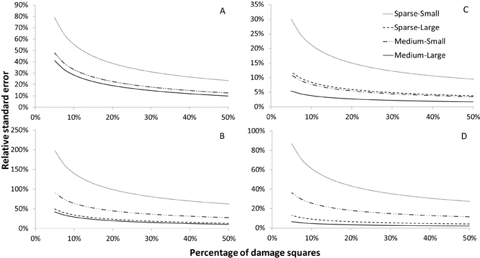
Fig. 2. Relative standard errors of estimators of the number of damaged trees ha–1 at a subsequent time point (TP2) (subfigs. A and C) and the increase, small and large increment, between the initial time point (TP1), at sparse and medium level, and TP2 (subfigs. B and D) for Scenario 1. Subfigures A and B show results obtained when using a sample consisting of a single year’s panel (n = 100), while subfigures C and D show results obtained using the full sample (N = 500).
Scenario 2 was designed to mimic local or regional outbreaks in which damage initially occurs in small groups of trees and then spreads rapidly. In this case, the relationship between the number of damaged trees ha–1 and the relative SE was less clear than in Scenario 1. The difference in relative SE between the sub-scenarios was relatively small for any given proportion of damage-containing squares. The precision of the estimators for the simulated populations was also clearly worse than in Scenario 1: the relative SEs exceeded 20 % in all cases, for both the estimator of the state in TP2 and the estimator of the increment, even when the full sample was utilized.
Fig. 3 shows the relative SEs of the estimators in relation to the actual number of damaged trees ha–1 resulting from each combination of sub scenario and percentage of squares containing damaged trees. For Scenario 1 and the low level of damage at TP1, i.e. 1.5 damaged trees ha–1 in squares containing damage, the relative SE was never less than 10 % even when the full sample was utilized (Fig. 3A). With this starting intensity of damaged trees, the relative SE of the estimator of the increase was less than 10 % when utilizing the full sample size if number of damaged trees ha–1 increased by more than 0.8. This figure corresponds to a relative increment of 50% in the case where all squares contain damaged trees, and a 200% increase in the case where 25% of all squares contain damaged trees. For the medium level of tree damage (in terms of damaged trees ha–1 at TP1), i.e. 12 damaged trees ha–1 in squares containing damaged trees, the relative SE was below 10% in almost all cases (Fig. 3B). As in the previous sub-scenario, increasing the number of damaged trees by 0.8 new trees ha–1 yielded a relative SE of less than 10 % when using the full sample. This corresponds to a relative increment of only 5 % of the starting level in the case where all squares initially contain damaged trees.
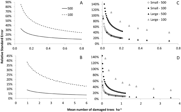
Fig. 3. Relative standard errors of estimators of the state at the initial time point (TP1; subfigs. A and B) and the increment, small and large, from TP1 to a subsequent time point (TP2; subfigs. C and D) in relation to the number of damaged trees ha–1 in Scenario 1 for the sparse (subfigs. A and C) and medium (subfigs. B and D) levels of tree damage at TP1. Results are shown for the full sample (N = 500) and a single year’s panel (n = 100).
When using only a single year’s panel, the standard errors of the estimators were greater in the sub-scenarios with larger increments between TP1 and TP2 for any given initial number of damaged trees ha–1. This shows that in a damage outbreak with a relatively high degree of aggregation, the number of damaged trees ha–1 will be less precisely estimated than in a more evenly-distributed outbreak involving the same number of damaged trees (Fig. 3). When the full sample is utilized, i.e. all squares are sampled, the increment had no effect on the SE of the estimators when starting with a random distribution of damaged trees as in Scenario 1. However, in Scenario 2, the SE for any given initial number of damaged trees ha–1 remains greater when considering larger increments or fewer damage-containing squares even when working with the full sample.
In Scenario 1, the power to detect an increment of a given size, i.e. to reject the null hypothesis of an increment of 1 tree ha–1 or less, was greater than 80 % when the actual increment was around 1.5 new damaged trees ha–1 and the full sample size was used (Fig. 4). With a single-year panel, a power of 80% was achieved for increments of around 2.3 trees ha–1 in cases involving a sparse distribution of damage at TP1 and a large increment between TP1 and TP2 (Fig. 4A). The power was lower with this number of trees ha–1 in the case involving an medium initial damage intensity and a large increment because under these conditions, there was more extensive aggregation of damage in a smaller number of squares (Fig. 4C). In the sub-scenarios involving small increments, the number of damaged trees did not increase by more than 1.2 tree ha–1 and so the probability of accurately identifying an increment of more than 1 was low.
In Scenario 2, with the sparse level of damage at TP1 and a small increment, a power of 80% was achieved for increments of approximately 3 damaged trees ha–1 when the full sample size was used (Fig. 4B). For the sub-scenarios involving an medium initial level of damage at TP1, a power of 80% was reached only if the actual increment was at least 15 trees ha–1 when using the full sample, or 56 damaged trees ha–1 when using a single year’s panel (Fig. 4D).
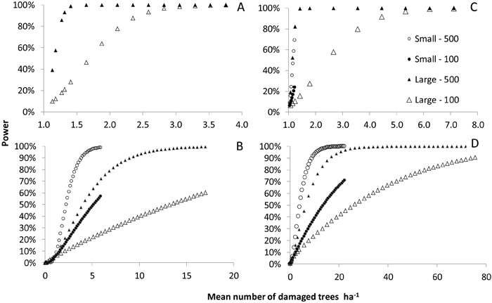
Fig. 4. The power to detect an increase in the number of damaged trees per hectare that exceeds 1 new damaged tree ha–1 in Scenario 1 (subfigs. A and C) and Scenario 2 (subfigs. B and D). Subfigs. A and B show the results for the sub-scenario with a sparse initial damage level while subfigs. B and D show the results for the sub-scenario with an intermediate initial damage level. Results are shown for a small and a large increment between the initial time point (TP1) and a subsequent time point (TP2). Data for the sub-scenario involving a small increment between TP1 and TP2 are omitted in the left hand figure, since the increase never exceeded 1 tree ha–1 in this case.
4 Discussion
The results obtained in this work show that sparse NFI-type inventories are capable of providing reliable information on forest state and damage outbreaks when these affect large areas at moderate to high damage intensities. This is consistent with previous findings by Wulff et al. (2006) and Nevalainen et al. (2010). However, in cases involving less intense outbreaks or highly aggregated outbreaks, it is clear that estimates based on NFI-type inventories have poor precision and will thus not generally provide a reliable basis for outbreak mitigation activities. This conclusion is similar to that drawn by Fisher et al. (2008), who showed that large but clustered events are more difficult to assess. Further, for most cases considered in our study, the estimates only had an acceptable level of precision when based on the whole sample. For certain types of damage, such as diseases that cause decay and develop slowly, estimates can be made based on data gathered over a period of several years. For other type of damage whose intensity peaks over a short period of time, such estimates will be much less meaningful. These differences in the scope for precise estimation of the extent of damage emphasize the importance of being clear about information needs and their relationship to different spatial scales (Wulder et al. 2006).
Our results indicate that the type of damage dispersal that can be expected in cases where damage accumulates over a long period of time can be estimated with satisfactory precision within a large scale monitoring program. It is therefore important to recognize and highlight the utility of large-scale monitoring programmes for monitoring damage of this type. For diffuse damage symptoms, which include those caused by climate change (e.g. drought damage), estimates from an NFI-type inventory are very useful. Climate change has the potential to create novel disturbances whose incidence may be scattered, and it is very important to update the effects of forest damage when performing risk assessments for management plans (Dale et al. 2001). To detect damage increases of this type, the long time series typically provided by an NFI type inventory are crucial. Other examples of damage types that might be well captured in NFI type inventories using the entire sample and moving averages are rot damage and game browsing (Swedish statistical yearbook… 2011). NFI data are currently used to model the probability of root rot damage (Thor et al. 2005; Mattila and Nuutinen 2007) and also to predict the probability of wind damage based on data for multiple years (Valinger and Fridman 1999; Peltola et al. 2010). However, when estimating the effects of a severe storm, it would be preferable to use only data from a single year´s panel. As such, damage events of this type are more difficult to capture within large scale inventories. The precision of the estimates obtained in such cases could potentially be improved by combing satellite imagery with large scale forest inventory data (Nelson et al. 2009). Other types of damage that one might want to monitor using NFI-type inventories include unforeseen forest disturbances caused by silvicultural or environmental changes.
Simulated sampling in artificial population is a useful tool for the evaluation of sampling strategies since many scenarios can be studied and the effects of different factors can be separated. However, the scope for drawing wider conclusions from the results depends on how accurately the artificial populations mimic real outcomes. In this study, two main damage scenarios were simulated as a basis for the design evaluations. They were chosen to describe realistic developments of forest damage, including the consideration that very few types of damage strike all kinds of forest over a large area (Edmonds et al. 2000). The latter issue was handled by varying the proportion of squares containing damaged trees. In Scenario 1, which involved a random dispersal of damage, the estimates obtained had comparatively low standard errors, especially in cases involving a large number of damaged trees ha–1. However, when damage is widely dispersed, random dispersal might be unrealistic since extensive dispersal almost always involves clusters of damage in real forests. Therefore, outbreaks involving large numbers of damaged trees are probably better described by Scenario 2. Conversely, when the number of damaged trees is low, the effect of clustered dispersion is negligible and Scenario 1 provides an adequate description of the spread of the damage.
All of the trees in each sample plot were included because the study was designed to explore the scope for monitoring a wide range of damage events. The real damage events mentioned when describing the two scenarios provide real-world examples of events with different damage intensities that are of general interest. The estimated standard errors obtained were relatively high. Data on resin-top disease, which was used as an example of low-frequency damage outbreaks, and on the Gremmeniella outbreaks that were used as examples of high frequency damage events, are typically collected by monitoring sample trees, as is done in all other types of damage assessment. In NFI-type inventories, sample trees are often selected at random from the entire set of trees on the sample plot (Lawrence et al. 2010). The relative standard errors are thus generally higher in estimates based on sample trees than for those based on every tree within the sample plot. Severe damage that causes tree death is recorded on all trees on the sample plot and should result in estimates with higher precision.
5 Conclusions
Considerable effort is invested into monitoring forest damage. The effectiveness of monitoring programmes and their ability to meet current and future needs have been discussed at length in the literature (Percy and Ferretti 2004; Lovett et al. 2007; Moffat et al. 2008). There is no doubt that forest damage monitoring is facilitated by a stable environment, but an ability to adapt to future needs is essential. The results presented in this work show that intermediate and large damage outbreaks in which damage occurs at random are likely to be well-captured by NFI-type inventories, but scattered damage outbreaks and outbreaks in which the number of damaged trees increases slowly between measurement occasions yield estimates with poor precision. We therefore propose that there may be a need to revise current forest damage monitoring programmes to make them more useful for monitoring the kinds of damage that are likely to arise as a consequence of climate change (Wulff et al. 2012).
Acknowledgement
Cornelia Roberge and Anna Hedström Ringvall were supported by grant 2008-546 from Formas. Insightful suggestions and comments were received from two anonymous referees.
References
Alexander C.J., Holland J.M., Winder L., Woolley C., Perry J.N. (2005). Performance of sampling strategies in the presence of known spatial patterns. Annals of Applied Biology 146(3): 361–370. http://dx.doi.org/10.1111/j.1744-7348.2005.040129.x.
Apollonio M., Andersen R., Putman R. (eds.). (2010). European ungulates and their management in the 21st century. Cambridge University Press. ISBN 978-0-521-76061-4.
Axelsson A.-L., Ståhl G., Söderberg U., Pettersson H., Fridman J., Lundström A. (2010). National Forest Inventories reports: Sweden. In: Tomppo E. et al. (eds.). National Forest Inventories: pathways for Common Reporting. 1st. ed. Springer. p. 613–621. ISBN 978-90-481-3232-4.
Baffetta F., Corona P., Fattorini L. (2011). Assessing the attributes of scattered trees outside the forest by a multi-phase sampling strategy. Forestry 84(3): 315–325. http://dx.doi.org/10.1093/forestry/cpr015.
Bechtold W.A., Pattersson P.L. (eds.). (2005). The enhanced forest inventory and analysis program-national sampling design and estimation procedure. General Technical Report SRS-80. U.S. Department of Agriculture, Forest Service, Southern Research Station.
Cochran W.G. (1977). Sampling techniques. New York. Wiley. ISBN 047116240X,9780471162407.
Dale V.H., Joyce L.A., McNulty S., Neilson R.P., Ayres M.P., Flannigan M.D., Hanson P.J., Irland L.C., Lugo A.E., Peterson C.J., Simberloff D., Swanson F.J., Stocks B.J., Wotton B.M. (2001). Climate change and forest disturbances. Bioscience 51(9): 723–734. http://dx.doi.org/10.1641/0006-3568(2001)051[0723:CCAFD]2.0.CO;2.
Dunn R., Harrison A.R. (1993). 2-dimensional systematic-sampling of land-use. Applied Statistics-Journal of the Royal Statistical Society Series C 42(4): 585–601.
Edgar C.B., Burk T.E. (2006). A simulation study to assess the sensitivity of a forest health monitoring network to outbreaks of defoliating insects. Environmental Monitoring and Assessment 122(1–3): 289–307. http://dx.doi.org/10.1007/s10661-005-9181-6.
Edmonds R.L., Agee J.K., Gara R.I. (2000). Forest health and protection. McGraw-Hill Higher Education. ISBN 0-07-021338-0.
Ferretti M. (1997). Forest health assessment and monitoring – issues for consideration. Environmental Monitoring and Assessment 48(1): 45–72. http://dx.doi.org/10.1023/A:1005748702893.
Ferretti M. (2009). Quality assurance in ecological monitoring-towards a unifying perspective. Journal of Environmental Monitoring 11(4): 726–729. http://dx.doi.org/10.1039/b902728a.
Fisher J.I., Hurtt G.C., Thomas R.Q., Chambers J.Q. (2008). Clustered disturbances lead to bias in large-scale estimates based on forest sample plots. Ecology Letters 11(6): 554–563. http://dx.doi.org/10.1111/j.1461-0248.2008.01169.x.
Forestry statistics 2010. (2010) Official Statistics of Sweden. Swedish University of Agricultural Sciences, Umeå. ISSN 0280-0543.
FutMon, Life+ EU. (2011). http://www.futmon.org/. [Cited 30 September 2011].
Gregoire T.G., Valentine H.T. (2008). Sampling strategies for natural resources and the environment. Chapman & Hall/CRC, Boca Raton. ISBN 1584883707, 9781584883708.
Jonsson M. (2008). Live-storage of Picea abies for two summers after storm felling in Sweden. Silva Fennica 42(3): 413–421.
Långström B., Lindelöw Å., Schroeder M., Björklund N., Öhrn P. (2009). The spruce bark beetle outbreak in Sweden following the January storms in 2005 and 2007. In: Kunca A. Zubrik M. (eds.). Insects and fungi in storm areas. Proceedings of the IUFRO Working Party 7.03.10 Methodology of Forest Insect and Disease Survey in Central Europe from the workshop that took place on September 15 to 19, 2008 in Štrbské Pleso, Slovakia. p. 13–19.
Lawrence M., McRoberts R.E., Tomppo E., Gschwanter T., Gabler K. (2010). Comparisons of national forest inventories. In: Tomppo E. et al. (eds.). National forest inventories: pathways for common reporting. Springer. p. 19–33. ISBN 978-90-481-3232-4. http://dx.doi.org/10.1007/978-90-481-3233-1_2.
Legendre P., Dale M.R.T., Fortin M.J., Gurevitch J., Hohn M., Myers D. (2002). The consequences of spatial structure for the design and analysis of ecological field surveys. Ecography 25(5): 601–615. http://dx.doi.org/10.1034/j.1600-0587.2002.250508.x.
Lorenz M. (1995). International co-operative programme on assessment and monitoring of air pollution effects on forests – ICP forests. Water Air and Soil Pollution 85(3): 1221–1226. http://dx.doi.org/10.1007/BF00477148.
Lovett G.M., Burns D.A., Driscoll C.T., Jenkins J.C., Mitchell M.J., Rustad L., Shanley J.B., Likens G.E., Haeuber R. (2007). Who needs environmental monitoring? Frontiers in Ecology and the Environment 5(5): 253–260. http://dx.doi.org/10.1890/1540-9295(2007)5[253:WNEM]2.0.CO;2.
Mattila U., Nuutinen T. (2007). Assessing the incidence of butt rot in Norway spruce in southern Finland. Silva Fennica 41(1): 29–43.
McRoberts R.E., Hansen M.H., Smith W.B. (2010a). National forest inventories reports: United States of America. In: Tomppo E. et al. (eds.). National forest inventories: pathways for common reporting. Springer. p. 569–580. ISBN 978-90-481-3232-4.
McRoberts R.E., Tomppo E.O., Naesset E. (2010b). Advances and emerging issues in national forest inventories. Scandinavian Journal of Forest Research 25(4): 368–381. http://dx.doi.org/10.1080/02827581.2010.496739.
Moffat A.J., Davies S., Finer L. (2008). Reporting the results of forest monitoring – an evaluation of the European forest monitoring programme. Forestry 81(1): 75–90. http://dx.doi.org/10.1093/forestry/cpm046.
Nelson M.D., Healey S.P., Moser W.K., Hansen M.H. (2009). Combining satellite imagery with forest inventory data to assess damage severity following a major blowdown event in northern Minnesota, USA. International Journal of Remote Sensing 30(19): 5089–5108. http://dx.doi.org/10.1080/01431160903022951.
Nevalainen S. (1999). Gremmeniella abietina in Finnish Pinus sylvestris stands in 1986–1992: a study based on the National Forest Inventory. Scandinavian Journal of Forest Research 14(2): 111–120. http://dx.doi.org/10.1080/02827589950152836.
Nevalainen S., Lindgren M., Pouttu A., Heinonen J., Hongisto M., Neuvonen S. (2010). Extensive tree health monitoring networks are useful in revealing the impacts of widespread biotic damage in boreal forests. Environmental Monitoring and Assessment 168(1–4): 159–171. http://dx.doi.org/10.1007/s10661-009-1100-9.
Oliva J., Thor M., Stenlid J. (2010). Long-term effects of mechanized stump treatment against Heterobasidion annosum root rot in Picea abies. Canadian Journal of Forest Research 40(6): 1020–1033. http://dx.doi.org/10.1139/X10-051.
Peltola H., Ikonen V.P., Gregow H., Strandman H., Kilpelainen A., Venalainen A., Kellomaki S. (2010). Impacts of climate change on timber production and regional risks of wind-induced damage to forests in Finland. Forest Ecology and Management 260(5): 833–845. http://dx.doi.org/10.1016/j.foreco.2010.06.001.
Percy K.E., Ferretti M. (2004). Air pollution and forest health: toward new monitoring concepts. Environmental Pollution 130(1): 113–126. http://dx.doi.org/10.1016/j.envpol.2003.10.034.
Russek-Cohen E., Christman M.C. (2004). Statistical methods for environmental monitoring and assessment. In: Wiersma B.G. (ed.). Environmental monitoring. CRC Press, Boca Raton. p. 391–406. ISBN 1-56670-641-6.
Särndal C.-E., Swensson B., Wretman J. (1992). Model assisted survey sampling. New York Springer-Verlag. ISBN 0-387-40620-4. http://dx.doi.org/10.1007/978-1-4612-4378-6.
Schreuder H.T., Gregoire T.G., Weyer J.P. (2001). For what applications can probability and non-probability sampling be used? Environmental Monitoring and Assessment 66(3): 281–291. http://dx.doi.org/10.1023/A:1006316418865.
Shaw J.D. (2008). Benefits of a strategic national forest inventory to science and society: the USDA Forest Service Forest Inventory and Analysis program. Iforest-Biogeosciences and Forestry 1: 81–85. http://dx.doi.org/10.3832/ifor0345-0010081.
Swedish statistical yearbook of forestry. (2011). Swedish Forest Agency. Jönköping. ISBN 978-91-88462-95-4.
Thor M., Stahl G., Stenlid J. (2005). Modelling root rot incidence in Sweden using tree, site and stand variables. Scandinavian Journal of Forest Research 20(2): 165–176. http://dx.doi.org/10.1080/02827580510008347.
Tomppo E., Gschwantner T., Lawrence M., McRoberts R.E. (eds.). (2010). National Forest Inventories – pathways for common reporting. Springer Science+Business media B.V. ISBN 978-90-481-3232-4.
USDA National Forest health Monitoring. USDA Forest Service. (2011). http://www.fhm.fs.fed.us/. [Cited 30 September 2011].
Valinger E., Fridman J. (1999). Models to assess the risk of snow and wind damage in pine, spruce, and birch forests in Sweden. Environmental Management 24: 209–217. http://dx.doi.org/10.1007/s002679900227.
Wulder M.A., Dymond C.C., White J.C., Leckie D.G., Carroll A.L. (2006). Surveying mountain pine beetle damage of forests: a review of remote sensing opportunities. Forest Ecology and Management 221(1–3): 27–41. http://dx.doi.org/10.1016/j.foreco.2005.09.021.
Wulff S. (2004). Nonsampling errors in ocular assessments. In: Wiersma B.G. (ed.). Environmental monitoring. CRC Press, Boca Raton. p. 337–346. ISBN 1-56670-641-6. http://dx.doi.org/10.1201/9780203495476.ch13.
Wulff S., Hansson P., Witzell J. (2006). The applicability of national forest inventories for estimating forest damage outbreaks – experiences from a Gremmeniella outbreak in Sweden. Canadian Journal of Forest Research 36(10): 2605–2613. http://dx.doi.org/10.1139/x06-148.
Wulff S., Lindelow A., Lundin L., Hansson P., Axelsson A.L., Barklund P., Wijk S., Stahl G. (2012). Adapting forest health assessments to changing perspectives on threats-a case example from Sweden. Environmental Monitoring and Assessment 184(4): 2453–64. http://dx.doi.org/10.1007/s10661-011-2130-7.
Zar J.H. (1999). Biostatistical analysis. 4th ed. Prentice Hall, Upper Saddle River, New Jersey. ISBN 0-13-082390-2.
Zarnoch S.J., Bechtold W.A. (2000). Estimating mapped-plot forest attributes with ratios of means. Canadian Journal of Forest Research 30(5): 688–697. http://dx.doi.org/10.1139/x99-247.
Total of 47 references
Appendices
Appendices 1 and 2 are downloadable at http://www.silvafennica.fi/supp_files/article1000/appendices.pdf.
