Petteri Seppänen  ,
Antti Mäkinen
,
Antti Mäkinen
Comprehensive yield model for plantation teak in Panama
Seppänen P., Mäkinen A. (2020). Comprehensive yield model for plantation teak in Panama. Silva Fennica vol. 54 no. 5 article id 10309. https://doi.org/10.14214/sf.10309
Highlights
- Tree level teak stem volume models, taper model and three sets of stand level yield models were developed using large empirical datasets
- Tree volume models were satisfactorily validated against independent measurement data and other published models
- Tree height as input parameter improved the stem volume model marginally
- Stand level yield models produced comparable harvest volumes with models published in the literature
- Stand level timber product outputs were found like actual harvests with an exception that the models marginally underestimate the share of logs in very large diameter classes.
Abstract
The purpose of this study was to prepare a comprehensive, computerized teak (Tectona grandis L.f) plantation yield model system that can be used to describe the forest dynamics, predict growth and yield and support forest planning and decision-making. Extensive individual tree and permanent sample plot data were used to develop tree-level volume models, taper curve models and stand-level yield models for teak plantations in Panama. Tree volume models were satisfactorily validated against independent measurement data and other published models. Tree height as input parameter improved the stem volume model marginally. Stand level yield models produced comparable harvest volumes with models published in the literature. Stand level volume product outputs were found like actual harvests with an exception that the models marginally underestimate the share of logs in very large diameter classes. The kind of comprehensive model developed in this study and implemented in an easy to use software package provides a very powerful decision support tool. Optimal forest management regimes can be found by simulating different planting densities, thinning regimes and final harvest ages. Forest practitioners can apply growth and yield models in the appropriate stand level inventory data and perform long term harvest scheduling at property level or even at an entire timberland portfolio level. Harvest schedules can be optimized using the applicable financial parameters (silviculture costs, harvesting costs, wood prices and discount rates) and constraints (market size and operational capacity).
Keywords
simulation;
teak;
decision support system;
Tectona grandis;
Panama;
taper curve;
volume equation;
yield model
-
Seppänen,
Verdas Oy, Kihlinkuja 7, FI-50600 Mikkeli, Finland
E-mail
petteri@verdas.fi
- Mäkinen, Simosol Oy. Hämeenkatu 10, FI-11100 Riihimäki, Finland E-mail antti.makinen@simosol.fi
Received 23 January 2020 Accepted 14 October 2020 Published 20 October 2020
Views 65255
Available at https://doi.org/10.14214/sf.10309 | Download PDF

Supplementary Files
1 Introduction
1.1 Modelling forest trees and stands
Planted forests are a valuable biological resource and the primary source of high-quality raw material for various industries. In forest management planning we need to understand and predict the dynamics and growth of the forests. This can be done using statistical models that describe the evolution of trees and forests, and computerised implementations of these models in forest simulators.
Starting with individual trees, their dimensions are modelled typically using empirical height- dbh and taper curve models. These models are commonly used in inventory calculations and for estimating the different commercial product volumes from the trees.
Switching from individual trees to groups of trees, or forests, the modelling becomes more complicated. Earliest (and simplest) forest growth models were the yield tables, tabular representations of the attribute of interest, e.g. stand volume, at different ages. Yield tables are easy to use, but also too simplified as they are usually associated with just one management scenario. Growth models can be classified by the unit of simulation into, for example, stand-level models, diameter distribution models and spatial and aspatial tree-level models (Munro 1974). Stand-level models explain the dynamics of different stand attributes, such as average height, basal area, or total volume. Tree-level models explain the dynamics of individual trees within a forest stand. The spatial models account for the actual locations of the trees and the distances between neighbouring trees. Between the “pure” stand-level and tree-level models are the so-called size class, or diameter distribution models (Tomé and Burkhart 1989; Vanclay 1994). Besides these listed model types, there are, for example, transition matrix models and succession models (Buongiorno and Michie 1980; Shugart and West 1980). Furthermore, forest models can be classified into empirical models (Zeide 1993) and process-based models (Mäkelä et al. 2000).
Finally, the selection of the most suitable type of model depends on the available modelling data and the application of the model. Tree-level models are often preferred over stand-level models as the former can, at least in theory, explain the within stand dynamics better and because a stand is a less distinct biological entity than a single tree (Garcia 2001; Porté and Bartelink 2002). On the other hand, stand-level models are simpler, computationally efficient and, according to multiple reports, more accurate (Vanclay 1994; Atta-Boateng and Moser 2000; Burkhart 2003). But they cannot cope with complex silviculture (e.g. uneven-aged forestry, mixed-species stands). Often stand-level models are favoured over tree-level models because data required to develop a good tree-level model can be expensive to collect.
1.2 Existing teak models
Research on teak (Tectona grandis L.f.) modelling has been carried out mainly in Central America, Brazil, Tanzania and India. Relevant published single tree stem volume and shape models are listed in Table 1. The existing research is based on reasonably sized data sets, but due to the large variation in the growing conditions and management practices, application of the existing models in other plantations can be problematic.
| Table 1. Existing publications on single tree volume and stem shape models for teak. | |||
| Source | Region | Model Application | Modelling Dataset |
| Pérez and Kanninen (2003) | Costa Rica | Total and merchantable stem volume | 111 trees Age 2–47 years Diameter 2–59 cm |
| Malimbwi et al. (2005) | Tanzania | Total stem volume | - |
| van Zyl (2005) | Tanzania | Stem volume, height and form | 222 trees Diameter 8–79 cm Height 9–34 m |
| Figueiredo et al. (2006) | Brazil | Stem volume and profile | 159 trees Age 7–10 years |
| Pérez (2008) | Costa Rica | Total and merchantable stem volume | 25 trees Age 8–46 Diameter 9–55 cm |
| Reggiani (2009) | Brazil | Total stem volume | - |
| Figueiredo et al. (2014) | Brazil | Stem volume and height (a book with some 40 equations for teak volume and height) | - |
| Ribeiro (2014) | Brazil | Stem heartwood volume | 40 trees Diameter 10–35 cm Height 14–27 m |
| Fallas (2017) | Costa Rica | Total and merchantable stem volume of clonal teak trees | 306 trees Age 3–12 years Diameter 9–32 cm |
Like tree-level models, also stand-level growth and yield models for teak are concentrated on a few regions, namely Costa Rica and Brazil. Table 2 presents the most relevant existing publications on stand-level growth and yield models for teak. Growth and yield models from India or African countries are generally from lower yield sites and therefore not applicable in higher productivity sites in Panama. Some of the published models from Central and South America are applicable only for young plantation due to limited modelling data.
| Table 2. Existing publications on stand-level growth and yield models for teak. | ||||
| Source | Region | Model Application | Modelling Dataset | Comments |
| Nunifu (1997) | Ghana | Stand-level yield models for dominant height, diameter, basal area, volume and biomass. Weibull model for diameter distribution modelling. | 100 sample plots Age 3–40 years | Modelling data includes only low yield sites |
| Bermejo (2004) | Costa Rica | Yield models/tables based on dominant height development | 318 sample plots | Modelling data covers only first half of full rotation. |
| Drescher (2004) | Brazil | Stand-level yield models for mean diameter, dominant height, form factor, stocking, basal area and volume | 162 sample plots Age 2–10 years Diameter 8–21 cm Height 10–18 m | Modelling data covers only first half of full rotation. |
| Pérez and Kanninen (2005) | Costa Rica | Stand-level growth curves for mean diameter and dominant height as a function of age | 150 sample plots Age 1–47 years | |
| García el al. (2006) | Brazil | Diameter distribution models for early thinning simulations | 239 sample plots Age < 96 months | |
| Saraiva et al. (2006) | Brazil | Diameter distribution models for early thinning simulations | 239 sample plots Age < 96 months | Same data as in García et al. (2006) |
| Batista (2007) | Brazil | Dominant height model for young teak plantations | Age < 12 years | |
| Pérez (2008) | Costa Rica | Stand-level dominant height curve | 25 sample trees | |
| Tewari et al. (2014) | India | Stand-level growth curves for dominant height, mortality, basal area and volume | 22 sample plots with 3 consecutive measurements Age 11–38 years | |
1.3 Rationale for a comprehensive plantation teak model
Implementation of growth models into forest simulators is an essential step so that they can be used as a decision support tool. The typical decision-making situations where forest simulators are needed include, for example, updating past inventory data into present day, scheduling thinning and final harvests, projecting future wood flows and cash flows, or quantifying the carbon sequestration of the forest over time. The different tasks require different functionalities from the forest simulator.
Simple tasks, such as projecting forest growth can be done using growth models or yield curves. Simulating harvests requires adding to the system a module to predict the different products and increases the level of complexity. The different products or assortments can be estimated using regression models, or taper models and a cross-cutting simulator and a dynamic optimisation model (Näsberg 1985). Additional complexity is introduced when the model is used for scheduling harvests and other treatments using simulation and optimisation approaches. As the level of complexity in the system increases, the model implementation becomes more demanding.
Teak is a high-value hardwood with a medium to long rotation. Modelling the economics is crucial for any commercial plantation project, and for a high-value timber with a large number of product classes, this is not an easy task. Analysing and comparing different rotations, thinning programs and classifications of products requires a comprehensive model of the plantation. Long-term decision-making problems include optimising the forest operations under estate level constraints, for example, that enforce sustainability of wood flows. Also, short-term decision problems, such as planning the harvests and timber sales on an annual basis, require a comprehensive, dynamic model of the plantation. Incorrect or overly simplified models can lead to sub-optimal decisions and economical losses.
The purpose of this study was to prepare a comprehensive, computerized teak plantation yield model system that can be used to describe the forest dynamics, predict growth and yield and support forest planning and decision-making.
2 Material and methods
2.1 Study area
2.1.1 Climatic conditions
The study area is in Panama Este and Darién provinces in the Republic of Panama in Central America (Fig. 1). According to the Köppen-Geiger climate classification system, the location falls into class Aw (tropical wet savanna climate); with the driest month having precipitation less than 60 mm and less than 4% of the total annual precipitation.
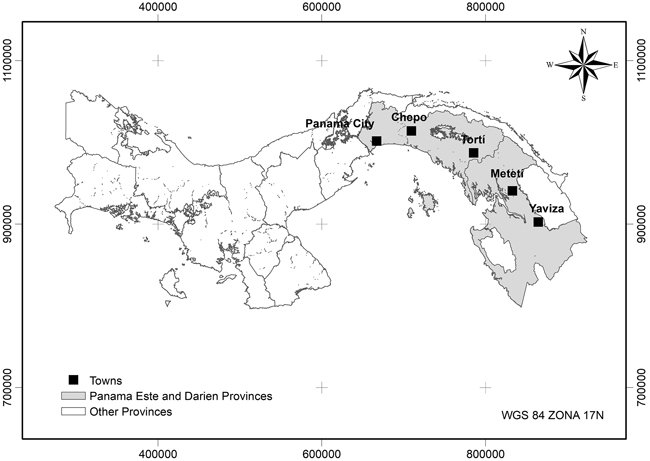
Fig. 1. Location of the teak growth and yield study area in Panama (Panama Este and Darien Provinces).
According to national public climate information, mean annual temperature (MAT) in the region oscillates between 26.5 and 27.2 degrees Celsius, being April the hottest month and December–January the coldest season. Total annual precipitation in the area averages 2000 mm year–1. Dry period with <50 mm of rainfall is three months from January to March as average. October is the wettest month with 300 mm of precipitation as average (Fig. 2.).
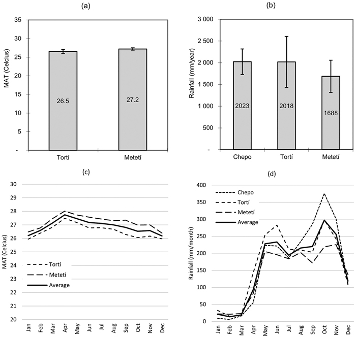
Fig. 2. Climate in different locations in the study area. Mean annual temperature and its standard deviation (graph a); total annual rainfall and its standard deviation (graph b); monthly average temperature (graph c); monthly average rainfall (graph d).
On the second half of the dry period in February–March, teak drops leaves. At the same time, tree growth ceases. The new rainy season in April–May kicks-on tree growth again. Often rainfall by mid-May is enough to start the new planting season, and the best plantations are those established in the beginning of the rainy season. It is generally agreed in the literature and forestry practice that teak requires a minimum of three months of dry period for high-quality wood formation. More extended dry periods would reduce the growth and yield; hence, three months is optimal.
2.1.2 Soil conditions
GIS data available in the region indicate vertisols and inceptisols being the most common soil types in the region. In general, soils have high clay content and deficient internal drainage capacity for forestry use. Table 3 provides a summary of 305 soil samples. Half of the samples represents 0–20 cm sampling depth and another half 20–40 cm. All soil samples were taken in teak plantations in the study area. The samples were analysed in the IDIAP (Instituto de Investigación Agropequaria) soil laboratory in Santiago, Panama.
| Table 3. Soil characteristics in teak plantations in the study area and teak optimum requirements for soil parameters as reported in published literature. | |||||||
| Soil Parameter | Unit | Method | N | Mean | St. Dev. | Teak Optimum | Source |
| Sand | % | Bouyoucos | 305 | 20% | 11% | 55…65% | (1) |
| Loam | % | Bouyoucos | 305 | 15% | 6% | … | … |
| Clay | % | Bouyoucos | 305 | 65% | 13% | 35...45% | (1) |
| Organic matter | % | Walkey-Black | 305 | 1.0% | 0.7% | 2.5…4.0+% | (1) |
| pH | NA | Water 1:2.5 | 305 | 6.1 | 0.6 | 5.5…6.2…7.2 | (1) |
| P | mg l–1 | Mehlich-1 | 305 | 10.2 | 20.1 | 3…10 | (1) (4) |
| K | mg l–1 | Mehlich-1 | 305 | 157 | 98 | >40…120+ | (1) |
| Ca | meq 100 g–1 | KCL | 305 | 23.1 | 13.2 | 1.5…4.0+ | (1) |
| Mg | meq 100 g–1 | KCL | 305 | 7.4 | 8.3 | 1.0…4.0 | (1) |
| Ca + Mg | meq 100 g–1 | KCL | 305 | 30.5 | 16.4 | 2.5…6.0+ | (1) |
| Al | meq 100 g–1 | KCL | 305 | 0.6 | 1.3 | <0.2 | (1) |
| CEC | meq 100 g–1 | Cation calculation | 305 | 31.7 | 16.2 | 4…10+ | (1) |
| Acid saturation | % | (Al + H)/CEC | 305 | 4% | 10% | <3…8% | (2) (3) (4) |
| Base saturation | % | (K + Ca + Mg)/CEC | 305 | 95% | 11% | n.a. | n.a. |
| Calcium saturation | % | Ca/CEC | 305 | 69% | 11% | >40...62…75% | (2) (3) (4) (5) |
| Teak optimum values according to: (1) Jerez and Coutinho (2017) (Brazil) (2) Alvarado and Fallas (2004) (Costa Rica) (3) Vaidés (2004) (Guatemala) (4) Mollinedo et al. (2005) (Panama) (5) Fernández-Moya et al. (2015) (Central America) | |||||||
Predominant soil texture in the study area is clay (98% in 0–20 cm samples and 97% in 20–40 cm samples are classified as clay soils) (Fig. 3). From a practical forestry perspective many soils in the region are often poorly drained being water filtration capacity the primary teak growth and yield limiting factor. Best teak plantations can be found in gentle hilly sites, where topography allows the excessive water surface run-off. Flat sites may have poor drainage which leads to anaerobic soil conditions in the rooting layer and, consequently, poor teak growth. In these sites, soil drainage needs to be improved with ditching and bedding for proper teak growth.
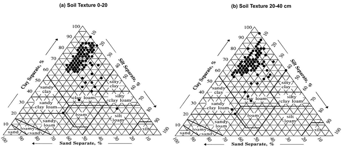
Fig. 3. Soil texture in teak plantations in the study area (n = 305). Clay, silt and sand separate were analysed on 0–20 cm and 20–40 cm sampling depths (graphs a and b respectively). View larger in new window/tab.
Soil chemical properties in the study area are characterised by high cation exchange capacity (CEC) (average over 30 meq 100g–1 of soil). Most of the CEC comes from calcium and hence calcium saturation of the soils is on the level required for good teak growth (>65%). Jerez and Coutinho (2017) report that a CEC of 4 meq 100g–1 in the soil is the minimum requirement and that a CEC over 10 meq 100g–1 is optimal for teak. Alvarado and Fallas (2004) report that teak needs 65% of calcium saturation and low acid saturation for good growth. Teak is very sensitive to aluminium. Practice in the study area has shown that aluminium content must be <1 meq 100g–1 for proper teak growth.
2.2 Stem volume and taper curve data
The data for individual tree models (stem volume equations and taper models) development was collected in connection with the first thinning and final felling operations in seedling plantations during 2013–2017. In felling sites a set of normally formed trees were randomly selected as sample trees. No leaning, forked, large buttress, or otherwise abnormal trees were sampled. Data collection of the felled trees was conducted by measuring stem diameter at 1.3 m above the stump (d) height and total stem height (h). Additional diameters were collected at 0%, 5%, 10%, 20%, 30%, 40%, 50%, 60%, 70%, 80%, 90% and 100% relative heights above the stump. All diameter measurements were collected with a diameter tape with an accuracy of 0.1 cm. In cases that a branch occurred in the diameter measurement point, then the measurement point was moved upwards along the stem, and the new relative height was recorded in the measurement data. Stem height was measured after felling with a measurement tape with an accuracy of 0.1 m until the tip of the stem. Stem volume between each diameter measurement point was calculated using the Smalian formula. The tip of the tree was calculated using the geometric cone formula. Total stem volume excluding stump was obtained by aggregating the individual “log volumes” between measurement points.
The dataset consists of 444 sample trees. After d/h plotting, 12 trees were eliminated for being clear outliers in the data due to measurement or recording errors. Hence, the final modelling dataset includes 432 sample trees. One hundred sixty-nine sample trees are from several first thinning sites across the study area. Thinning and measurement of d/h pairs along the stem was performed at age 5 in some 1500 ha. Two hundred sixty-three sample trees originated from final felling at age 20–22 years in some 400 ha and three different sites across the study area. One dummy tree (d = 1.0 cm; h = 1.5 m) was added in the data to make the model more realistic in very small diameter classes. In each model fitting, 50 trees were randomly re-sampled and used as validation data; hence, the model fittings were performed for 383 sample trees. Sample tree data is plotted in Fig. 4.
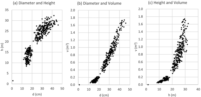
Fig. 4. Sample tree data relationships (n = 433) in stem volume and taper curve modelling dataset (d = stem diameter at 1.3 m height, h = stem height).
2.3 Yield model data
Sample plot data (n = 2634) used in this study has been collected from permanent sample plots in Panama during 1996–2017 in seedling plantations across 23 plantation sites in the study area in Panama Este and Darien provinces. Plots were circular with an area of 500 m2. In each plot, stem diameter and total height of all the trees were measured on an annual basis. The dataset includes 311 individual plots that were re-measured 1–19 times (8.5 re-measurements per plot as average). The data are well balanced in terms of age classes and site indices, i.e. both young/mature, and low/high site index sites are represented in the data (Table 4). This allows non-biased model fitting. Average site index in the dataset is 25.5 meters. Half of the sample plots (48%) represent Site Index values lower than 25.5 meters and another half (52%) above 25.5 meters. The data covers an age range of 1.5–20 years (Table 5, Supplementary file S1).
| Table 4. Number of sample plots in the yield model dataset. | |||
| Age | SI20 < 25.5 | SI20 > 25.5 | Total n |
| <10 | 791 | 971 | 1762 |
| >10 | 472 | 400 | 872 |
| Total n | 1263 | 1371 | 2634 |
| Table 5. Stand parameter summary in the yield model dataset. | ||||||||||
| Parameter | Age | D | Dmax | Dmin | H | Hd | N | G | V | SI20 |
| Min | 1.5 | 3.7 | 4.7 | 0.5 | 3.2 | 3.5 | 20 | 0.2 | 1.2 | 9.5 |
| Max | 19.9 | 43.3 | 54.4 | 39.0 | 29.9 | 30.3 | 1260 | 28.0 | 312.2 | 42.6 |
| Mean | 8.9 | 20.3 | 24.1 | 15.6 | 17.4 | 18.0 | 441 | 11.2 | 98.8 | 25.5 |
| Median | 7.7 | 20.4 | 24.2 | 15.9 | 17.8 | 18.3 | 360 | 11.3 | 95.9 | 25.6 |
| D = mean diameter (cm); Dmax, Dmin = maximum and minimum diameters (cm); H = mean height (m); Hd = Dominant height (m); N = stocking (trees ha–1); G = basal area (m2 ha–1); V = total stem volume (m3 ha–1); SI20 = Dominant height at base age of 20 years (m). | ||||||||||
2.4 Stem volume and taper curve model estimation
Altogether 35 different equations were fitted in the modelling dataset, of which 14 equations were single-entry models v = f(d) and 21 were double-entry v = f(d, h) (v denotes for total stem volume).
The taper curve equation selected for this study was an 8th-degree polynomial. These types of polynomial equations have been utilised widely for modelling tree stem shape, for example by Laasasenaho (1982). Other types of tree taper models and approaches have been discussed extensively in Burkhart and Tomé (2012). Teak stem form has been studied by zan Zyl (2005) and Figueiredo (2006). Although the authors acknowledge that there is a number of alternative taper models available, the 8th degree polynomial was selected as its parametrisation is straightforward, and in this study its estimation statistics, as well as the residual plots, indicated that the polynomial model fitted the data well. Evaluating and comparing alternative taper models with this data set would constitute a separate study and a research report.
Data processing for stem volume equations and taper curve equation was performed using linear and non-linear regression. The candidate models were evaluated based on the coefficient of determination (R2), Root Mean Square Error (RMSE), residual average (bias) and residual plot graphs.
2.5 Yield model estimation
Three alternative model systems, named A, B and C, were fitted to the data set as the stand-level yield models. The selected model systems were based on previous studies on similar recursive yield model approaches by Eerikäinen (2002) and Kaura (2009). All three model systems are driven by stand age (t) and stocking (N, number of stems per hectare), and the dependent variables are Hd (dominant height, m), H (mean height, m), D (mean diameter at breast height, cm) and V (volume, m3 ha–1). Model systems B and C had also Dmax (maximum diameter), and G (basal area, m2 ha–1) as dependent variables. The model systems are so-called recursive regression models, where results of one model are used as input parameters in other models. The alternative model systems A, B and C have proved to be robust when fitting datasets from different species and regions.
Dominant height model is the two-parameter Chapman-Richards equation Hd = f(t). Mean height is predicted with logarithmic model H = f(Hd). Guide curve method was applied for the site index model. The guide curve is fitted in the Hd/t data and the obtained curve represents an average site index. Heights at all ages for other site classes are assumed to be proportional to the guide curve (Clutter et al. 1983; Burkard and Tomé 2012; Ribeiro et al. 2016).
Mean diameter model is also a logarithmic model D = f(N, t, Hd). Basal area is predicted with a logarithmic expression of G = f(N, D), and standing timber volume V = f(D, Hd, N) or V = f(N, G), depending on the model system. Tree heights are calculated with Näslund’s height equation h = d2/(B0+B1×d)2 (Näslund 1936). Diameter distribution of a stand is predicted using the Weibull probability density function and a parameter prediction method (Clutter et al. 1983). Scale parameter prediction model is a linear model Scale = f(D), and shape parameter model is a logarithmic expression Shape = f(D, Dmax).
The yield model parameters were estimated using Two-Stage Least Squares (2SLS) regression analysis technique. 2SLS is an extension of Ordinary Least Squares (OLS) estimation and is used when the error terms of the dependent variable are correlated with the independent variables, or if the model has feedback loops. The models were estimated using R’s systemfit package (Henningsen and Hamann 2007).
2.6 Forest simulator description
The forest simulator developed within this study uses single tree volume and taper curve models for inventory calculations, as well as for simulating the different products obtained from harvests.
The forest simulator was implemented in IPTIM Assets -software (Integrated Planning for Timberland Management, https://www.simosol.fi/assets-long-term-optimization). Iptim utilises SIMO (SIMulation and Optimisation framework, http://www.simo-project.org) for the actual simulation and optimisation tasks. The simulator includes a database module, a growth and yield module, harvest simulation and bucking module, silvicultural treatment module, as well as a built-in optimisation module. SIMO framework allows for easy implementation of different types of forest simulators and provides all the core functionalities required for a comprehensive forest planning system (Rasinmäki et al. 2008).
The term forest simulator covers in this study the full programmatic implementation of the various models within a forest planning system. Fig. 5 gives a conceptual, high-level overview of the system components and how the different models developed within this study are applied. The high-level overview follows a simple case study of scheduling harvests for several stands using a simulation and optimisation approach.
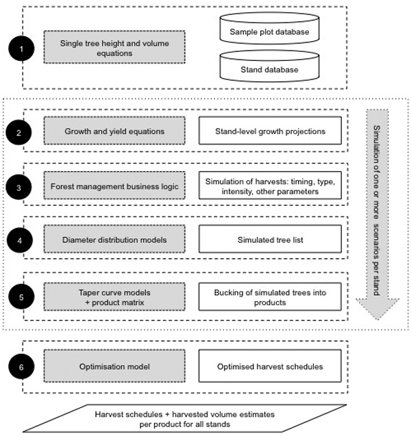
Fig. 5. Conceptual description of the forest simulator and optimisation model.
Step 1 inventory calculations utilise tree-level volume models for predicting the volumes for sample trees that have been inventoried for d and h. The tree-level inventory data collected from the sample plots are also used for estimating stand-level forest attributes for the actual management units or stands. Inventory calculations are used for estimating the current forest properties at sample plot, stand or property or portfolio-level. The inventory calculations can also be considered as a pre-processing or initialisation phase for the actual forest planning phase.
Step 2 utilises the growth and yield equations to project the development of stand-level attributes over a specific time period. The exact stand-level attributes that are projected vary between the different growth and yield models.
Step 3 covers the forest management business logic defined in the simulation logic. In this case, the most important business logic is related to the timing of thinning and final felling. Typically, also other treatments, such as regeneration and silvicultural actions, are programmed into the business logic.
Step 4 simulates a tree list using a size distribution model for a stand at the time of harvest. In this study, the size distribution models are based on a Weibull function. This means that the business logic of step 3 defines when the tree lists will be simulated.
Step 5 simulates the stem profile for each simulated tree from step 4 and optimises the cutting of the stem using a bucking model, in this case simple dynamic optimisation, and a product matrix that defines the minimum dimensions of all possible products as well as their values.
Steps 2 to 5 can be considered as the actual simulation phase. It can be repeated any number of times, and by varying the timings and other parameters of the harvests in step 3, it is possible to simulate many alternative harvest schedules for the optimisation phase.
Step 6 is the optimisation phase in which the optimiser selects a single harvest schedule for each stand so that the objective function is maximised (or minimised) and the solution conforms to possible estate-level constraints. In this study we did not formulate an actual optimisation problem, but in general the adopted approach allows for plugging in an optimisation model that can be used to set constraints on, for example, maximum annual harvest levels or even wood flow.
The forest planning system described here can be used for multiple forest planning tasks, such as inventory calculations, forest database updating, forest growth projections, harvest scheduling and cash flow modelling.
In summary, forest inventory data collected from sample plots, together with tree-level volume models, is used to produce estimates of the current growing stock attributes. Growth and yield models are used for projecting forest growth into the future. Forest management business logic describes how and when treatments are done. Stem diameter distribution model and taper curve model are used for modelling the product mix from harvests. Finally, the optimisation model is used for scheduling the harvests with given objective and constraints.
3 Results
3.1 Stem volume and taper curve models
Based on the statistical performance and residual plot graphs, two single-entry models and four double-entry models were selected (Table 6). Single entry models where stem volume is explained only with diameter, produced similar R2, RMSE and residual average than double-entry models where diameter and height are used as input parameter. Hence, the inclusion of tree height in the model did not significantly improve the overall model goodness of fit.
| Table 6. Selected single-entry and double-entry stem volume models. | |||||
| Model | Equation | N | R² | RMSE | Bias |
| D8 | 383 | 0.970 | 0.056 | –0.001 | |
| D10 | v = 8.2091 × exp(–70.331 / d) | 383 | 0.970 | 0.079 | +0.003 |
| DH21 | v = 0.000032589 × d2 × h | 383 | 0.974 | 0.074 | +0.011 |
| DH22 | v = 0.029387 + 0.000031543 × d2 × h | 383 | 0.973 | 0.073 | +0.000 |
| DH29 | v = 0.000078168 × d2 + 0.00020175 × (h – 1.3)2 + 0.000025461 × d2 × h – 0.0000000094597 × d × h2 | 383 | 0.978 | 0.068 | –0.005 |
| DH35 | v = 0.0028011 × d + 0.0059896 × (h – 1.3) + 0.000030872 × d2 × h | 383 | 0.978 | 0.066 | –0.003 |
| v = stem volume (m3); d = diameter at 1.3 m above the stump (cm); h = stem height (m). | |||||
Stem volume model fittings and model validation residual plot graphs are shown in Suppl. files S2 and S3. All the selected models show a random pattern in residuals; hence, they predict the stem volume without significant bias. When comparing single-entry and double-entry models, the latter have smaller residuals in small volume classes, and hence double-entry models can be considered marginally more accurate.
Comparison of the fitted models against other teak volume equations is shown in Fig. 6. The difference between the model performances is smaller with double-entry models than with single-entry models. This suggests that the d/h relationship is different in datasets obtained from different plantations with specific growing conditions, genetic material and management history. Interestingly, the model fitted to clonal sample trees by Fallas (2017) seem to perform in a similar manner with other models.
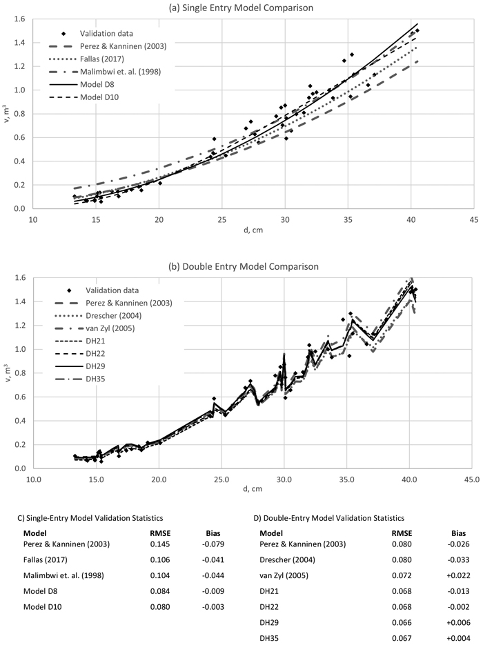
Fig. 6. Stem volume model validation with re-sampled data. Single-entry Models D8 and D10, and double-entry models DH21, DH22, DH29 and DH35 were the best performing models in this study. For details of the other published models, see Table 1 and Table 2. d = stem diameter at 1.3 m height and v = stem volume.
The taper equation has a good fit (R2 = 0.941), a low RMSE, a low average residual value and importantly, a negligible bias (Fig. 7, Suppl. file S4). According to earlier experience, as well as other research (for example Laasasenaho 1982), the 8th degree polynomial model is flexible and has worked well for various tree species. Hence no other types of taper curves were evaluated in this study.
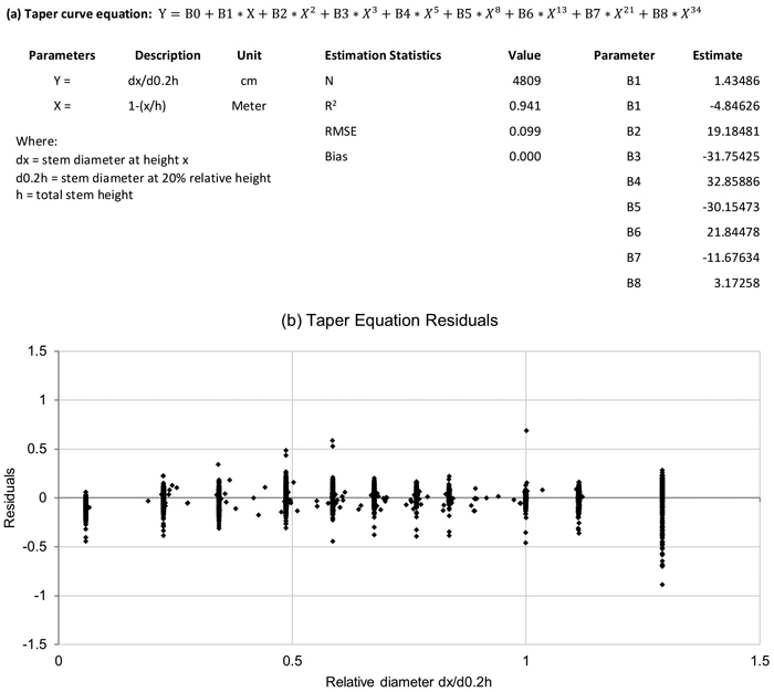
Fig. 7. Taper equation model (graph a) and residuals (graph b) (dx = diameter at height x; d0.2h = diameter at 20% relative height).
3.2 Stand level yield models
Yield model equations with regression coefficients and model fitting statistics are provided in Table 7. All models show good fitness in the dataset with high R2 and low bias and RMSE. Also, residual graphs are acceptable showing no correlation (Suppl. files S5–S8).
| Table 7. Summary of Yield Models A, B and C. View in new window/tab. |
Models A, B and C performance for mean diameter and total stem volume under a typical management regime (stocking 650-550-375-250 trees ha–1) is shown in Fig. 8. With low site index (SI = 20–25), all three models produce comparable results. On very productive sites with SI > 25, model A mean diameter development is significantly faster after mid-rotation than in case of models B and C. This turns into very high and probably un-realistic growing stock in the age range of 10–20 years.
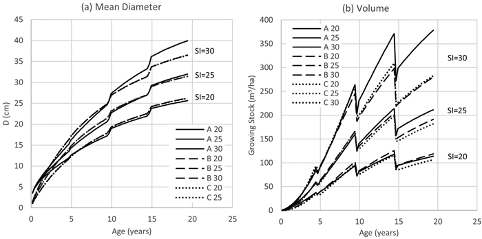
Fig. 8. Yield Model A, B and C performance with different Site Index values (D = stand mean diameter at 1.3 m height; V = stand total volume; SI = Site Index or dominant height with base age 20 years; A, B, C = volume models).
3.3 Forest management simulations
Forest management simulations were performed with Iptim. Yield Model B and C were applied in thinning regimes of Bermejo et al. (2004) and Perez and Kanninen (2005). Planting density is 1111 trees ha–1, and the thinning regime was defined by stocking (N ha–1). In thinning simulations, the stems were removed from the low-end of the diameter distribution until the prescribed stocking was achieved.
The regimes and harvest output volumes are shown below in Figs. 9 and 10. Harvest outputs, as estimated with Model B and Model C, produced comparable results with the benchmark studies. Simulation results suggest that Model B and Model C harvest outputs are possibly more sensitive to stocking that the benchmark models of Bermejo et al. (2004) and Perez and Kanninen (2005). Model B and Model C produced similar log size distributions.
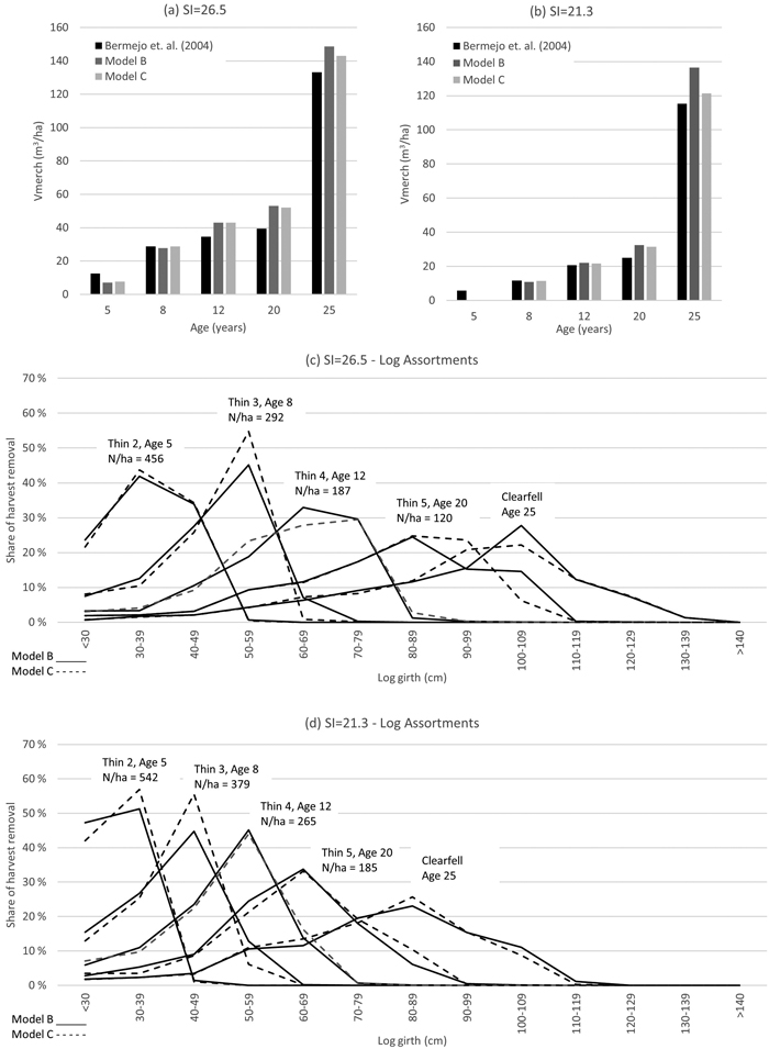
Fig. 9. Merchantable volume harvest output comparison with the study of Bermejo et al. (2004) with Site Index SI = 26.5 and SI = 21.3 (graphs a and b), and log assortments as estimated with Model B and Model C (graphs c and d).
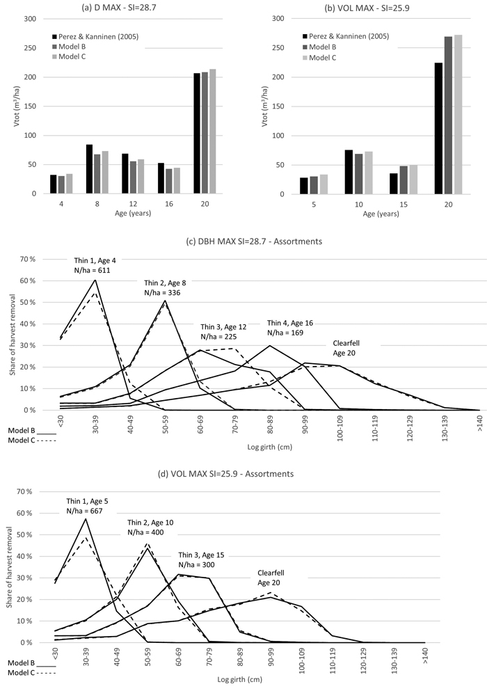
Fig. 10. Total volume harvest output comparison with the study of Perez and Kanninen (2005) with diameter maximization growth scenario (graph a) and total volume maximization growth scenario (graph b), and respective log assortments as estimated with Model B and Model C (graphs c and d).
3.4 Site index model validation
The modelled site index curve is shown in Fig. 11, together with other published teak site index models. The curve fitted in this study represents a somewhat average dominant height development over time. The model of Perez and Kanninen (2005) indicates slower height growth over time than other models, and the equations by Bermejo et al. (2003) and Drescher (2004) very fast height growth at the age of 1–5 years and then an early inflexion point. However, the studies of Bermejo et al. (2004) and Drescher (2004) include data only from young and mid-rotation plantations until the age of 10 years.
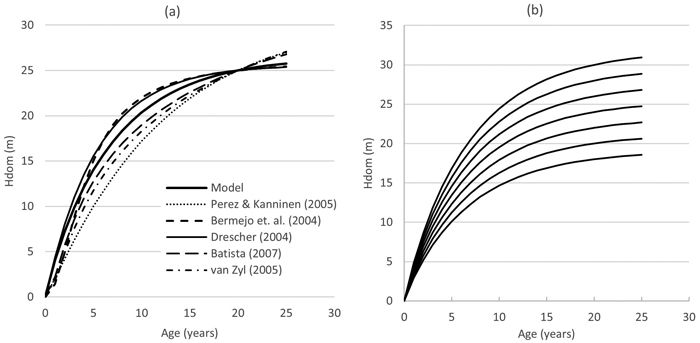
Fig. 11. Site Index curve comparison (graph a) and Model curve set for site indices 18–30 (graph b). Hd = dominant height.
All benchmarked site index models show that teak height growth is very fast during the first half of the rotation until the age of 10 years, reducing after that significantly towards final harvest at the age of 20–25 years; approximately 80% of teak’s height growth is achieved by mid-rotation.
3.5 Assortment distribution validation
Results from four case studies on estimated and actual log size comparison are shown in Fig. 12. Each graph corresponds to commercial scale teak final felling operation at the age of 20 years approximately, with a mean diameter of 31–33 cm. The stand parameters required for the diameter distribution and log size modelling (D, Dmax) were obtained from pre-harvest inventory before the harvest operation. Harvesting consisted of chainsaw felling and cross-cutting to 2.3-meter logs, extraction, and log-by-log timber scaling at log yard. Each harvest operation consisted of 5000–14 000 m3 of merchantable timber in girth classes 40–140 cm over bark. The results obtained from the case studies indicate that the model system with the Weibull diameter distribution and the taper curve application produces reliable results, provided that the model input parameters (D, Dmax) are accurate. However, in very large girth classes (110 cm and above) actual volumes were consistently larger than the model estimations.
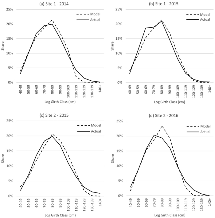
Fig. 12. Log size output comparisons (Model C predicted vs Actuals) in four final harvest operations in Panama.
4 Discussion
This study describes a comprehensive, computerised plantation forest model that can support decision making in forest management. Forest growers or managers are interested in issues such as stand parameter development over time, projected wood flows with given forest management prescriptions, harvested product mix as affected by timing of the thinning and final felling, or optimal harvest schedule over the entire rotation. Forest owners on the other hand could be interested, for example, in understanding the economic value of the forest. The fair value of the forest is often established using discounted cashflow method that is based on optimized harvest schedule.
As a part of the study, an extensive individual tree data set and permanent sample plot data set were used to develop tree-level volume models, taper curve models and stand-level yield models for teak plantations in Panama. Coefficients of determination of the fitted stem volume models were at a high level (around 0.97 for single entry models and 0.97–0.98 for double entry models) and residuals did not show tendency when plotted over the predicted tree volume. Inclusion of tree height in stem volume prediction improved the model fit only marginally – this could be due to little height variation in teak plantations that are grown with a standard stocking level. Stem volume models were compared with teak models from previous publications and were found to have comparable performance especially in double-entry models (Malimbwi 1998; Pérez and Kanninen 2003; Dreschler 2004; van Zyl 2005; Fallas 2017).
Stand level yield models had the following coefficients of determination: Dominant height 0.86; mean height 0.92, mean diameter 0.91 and stand volume 0.99. Residuals showed random pattern when plotted over predicted stand variables and hence the models are considered unbiased. As was evident also in previous studies by (Bermejo et al. 2004; Batista 2007), analysis of the teak height growth pattern indicated that 80% of the height growth is achieved by mid-rotation. This underlines the pioneering nature of teak as a tropical species.
When comparing the three estimated yield model sets (A, B and C), model set A was found to show faster mean diameter growth over time than models B and C. Consequently, model A produced likely overestimated volumes on very productive sites. Model sets B and C yielded comparable harvest volumes with other published studies under same site index and thinning regime (Perez and Kanninen 2005; Bermejo et al. 2014).
This study included three alternative growth and yield model systems, which the authors in previous modelling work have proved to be robust and having good fit with different datasets. However, it is possible that even better performing models could be identified in further studies.
The set of models applied in this study was estimated using permanent sample plot data from seedling plantations. It is important to note that the stem form and height development pattern in clonal plantations may differ from seedling plantations. As soon as tree-level and plot-level empirical data are available at least for ¾ of the planned rotation (i.e. 15 years), the tree volume and taper models should be re-estimated with the data from clonal trees, followed by a calibration of the yield models. In the meanwhile, in the absence of empirical tree-level and stand-level data from clonal plantations over the entire rotation, the models developed in this study can cautiously be used as a proxy when simulating clonal yields, because the most important yield driver, site index, is included in the model system as an independent variable. However, it should be kept in mind that the shape of the growth curve in clonal plantations may differ from seedling plantations. The model set is strongly driven by dominant height and stocking, which emphasises the need for accurate stand-level inventory data for these parameters.
One model component not considered in this study explicitly is natural mortality. Natural mortality can be accounted for in forest models using various approaches. Such approaches include logistic survival models for individual trees, mortality models based on the concept of maximum basal area carrying capacity and Reineke’s Stand Density Index (SDI). Mortality models based on the two latter approaches typically adjust the stocking of the stand downwards when the stand reaches a stocking or basal area that is higher than a given maximum level. In absence of the explicit mortality model, author’s experience is that a cautious 15% reduction in stocking could be applied in year 1 to account for initial mortality after planting, and further 0.5% annual stocking reduction until final harvest to allow for losses due to wind damages and lightning – both common phenomena in teak plantations in Panama.
The climatic and soil conditions are determinant for the site productivity. In this study the site index estimated for each stand is an implicit proxy for soil, climate and other factors affecting the growth potential. However, in Panama tree growth takes place mainly during rainy season between May and December and very little growth from January to April is achieved (dry season). The growth seasonality could be factored in the yield model system by allocating the annual growth to the rainy season only as a function of accumulated rainfall. This would further improve the accuracy of the harvest volume predictions.
The kind of comprehensive model developed in this study and implemented in an easy to use software package provides a useful decision support tool for plantation management.
References
Alvarado A., Fallas J.L. (2004). Efecto de saturación de acidez y encalado sobre el crecimiento de la teca (Tectona grandis Lf) en suelos ácidos de Costa Rica. [Effect of acid saturation and liming on growth of teak (Tectona grandis Lf) in acid soils in Costa Rica]. Agronomía Costarricence 28(1): 81–87. [In Spanish].
Atta-Boateng J., Moser J.W. (2000). A compatible growth and yield model for the management of mixed tropical rain forest. Canadian Journal of Forest Research 30(2): 311–323. https://doi.org/10.1139/x99-210.
Batista de Oliveira E. (2007). SisTeca – simulador de crescimento e produção para o manejo de plantações de Tectona grandis. [SisTeca – growth and yield simulator for the management of Tectona grandis plantations]. Comunicado Técnico 199. Colombo. 5 p. [In Portuguese].
Bermejo I., Cañellas I., San Miguel A. (2004). Growth and yield models for teak plantations in Costa Rica. Forest Ecology and Management 189(1–3): 97–110. https://doi.org/10.1016/j.foreco.2003.07.031.
Buongiorno J., Michie B.R. (1980). A matrix model of uneven-aged forest management. Forest Science 26(4): 609–625.
Burkhart H. (2003). Suggestions for choosing an appropriate level for modelling forest stands In: Amaro A., Reed D., Soares P. (eds.). Modelling forest systems. Workshop on the interface between reality, modelling and the parameter estimation processes, Sesimbra, Portugal, 2–5 June 2002. CABI Publishing, Oxfordshire. p. 3–10. https://doi.org/10.1079/9780851996936.0003.
Burkhart H., Tomé M. (2012). Modeling forest trees and stands. Springer. 446 p. https://doi.org/10.1007/978-90-481-3170-9.
Clutter J.L., Fortson J.C., Pienaar L.V., Brister G.H., BAiley R.L. (1983). Timber management: a quantitative approach. John Wiley & Sonsa. 333 p.
Drescher R. (2004). Crescimento e produção de Tectona grandis Linn F, em povoamentos jovens de duas regiões do estado de Mato Grosso – Brazil. Tese de Doutorado. Universidade Federal de Santa Maria. [Growth and yield of Tectona grandis Linn F in young plantations in two regions in Mato Grosso – Brazil. Doctoral Thesis. Federal University of Santa Maria]. 116 p. [In Portuguese].
Eerikäinen K. (2002). A site dependent simultaneous growth projection model for Pinus kesya plantations in Zambia and Zimbabwe. Forest Science 48(3): 518–529.
Fallas Zúñiga J.L. (2017). Funciones alométricas, de volumen y de crecimiento para clones de teca (Tectona grandis Lf) en Costa Rica. Tesis de Maestría. Escuela de Ingeniería Forestal. [Allometric functions, volume functions and growth functions for teak clones (Tectona grandis Lf) in Costa Rica. Master’s Thesis. School of Forest Engineering]. 69 p. [In Spanish].
Fernández-Moya J., Alvarado A., Mata R., Thiele H., Segura J.M., Vaides E., San Miguel-Ayanz A., Marchamalo-Sacristán M. (2015). Soil fertility characterization of teak (Tectona grandis Lf) plantations in Central America. Soil Research 53(4): 423–432. https://doi.org/10.1071/SR14256.
Figueiredo Filho A., Amaral Machedo S., Veiga de Miranda R.O., Souza Retslaff F.A. (2014). Compêndio de equações de volume e de afilamento de espécies florestais plantadas e nativas para as regiões geográficas do Brazil. [Compendium of volume and taper equations for planted and native forest species in geographical regions in Brazil]. Curitiba. [In Portuguese].
Figueiredo Orfanó E., Scolforo Soares J.R., Donizette de Oliveira A. (2006). Seleção de modelos polinomiais para representar o perfil e volume do fuste de Tectona grandis Lf. [Selection of polynomial models to represent stem form and stem volume of Tectona grandis Lf.]. Acta Amazonica 36(4): 465–482. https://doi.org/10.1590/S0044-59672006000400008. [In Portuguese].
Garcia O. (2001). On bridging the gap between tree-level and stand-level models. http://citeseerx.ist.psu.edu/viewdoc/download?doi=10.1.1.547.5687&rep=rep1&type=pdf. 12 p. [Cited 22 Dec 2019].
Garcia Leite H., Saraiva Nogueira G., Chagas Campos J.C., Hissashi Takizawa F., Lopes Rodrigues F. (2006). Um modelo de distribuição diamétrica para povoamentos de Tectona grandis submetidos a desbaste. [A diametric distribution model for thinned stands of Tectona grandis]. Revista Árvore 30(1): 89–98. https://doi.org/10.1590/S0100-67622006000100011. [In Portuguese].
Henningsen A., Hamann J. (2007). Systemfit: a package for estimating systems of simultaneous equations in R. Journal of Statistical Software 23(4): 1–40. https://doi.org/10.18637/jss.v023.i04.
Jerez-Rico M., de Andrade Coutinho S. (2017). Establishment and management of planted teak forests. In: Kollert W., Kleine M. (eds.). The global teak study. Analysis, evaluation and future potential of teak resources. IUFRO World Series 36. p. 49–65. https://www.iufro.org/publications/article/2017/06/21/world-series-vol-36-the-global-teak-study-analysis-evaluation-and-future-potential-of-teak-reso/.
Kaura E. (2009). Pinus patulan tuotosennusteiden tarkkuuden riippuvuus mallinnusaineiston koosta ja estimointitavasta: tapaus Tansania Sao Hill. [The effect of the data size and estimation method on the yield estimates of Pinus patula– case study in Tanzania Sao Hill]. Helsingin yliopisto, Maatalous-metsätieteellinen tiedekunta, Metsävarojen käytön laitos. 83 p. http://urn.fi/URN:NBN:fi:hulib-201507211654. [In Finnish].
Laasasenaho J. (1982). Taper curve and volume functions for pine, spruce and birch. Communicationes Instituti Forestalis Fenniae 108. 74 p. http://urn.fi/URN:ISBN:951-40-0589-9.
Mäkelä A., Landsberg J., Ek A.R., Burk T.E., Ter-Mikaelian M., Ågren G., Chadwick D.O., Puttonen P. (2000). Process-based models of forest ecosystem management: current state-of-art and challenges for practical implementation. Tree Physiology 20(5–6): 289–298. https://doi.org/10.1093/treephys/20.5-6.289.
Malimbwi R.E., Mugasha A.G., Chamshama S.A.O., Zahabu E. (1998). Volume tables for Tectona grandis at Mtibwa and Longuza forest plantations. Tanzania Sokoine University of Agriculture, Faculty of Forestry and Nature Conservation. Record no 71. Morogoro.
Mollinedo M., Ugalde L., Alvarado A., Verjans J.M., Rudy L.C. (2005). Relación suelo-arbol y factores de sitio, en plantaciones jóvenes de teca (Tectona grandis), en la zona oeste de la cuenca de Panama. [Relationship soil-tree and site factors in young teak (Tectona grandis) plantations in west of Panama watershed]. Agronomía Costarricense 29(1): 67–75. https://www.redalyc.org/pdf/436/43629107.pdf. [In Spanish].
Munro D.D. (1974). Forest growth models – a prognosis. Research Notes Royal College of Forestry 30. Stockholm. p 7–21.
Näsberg M. (1985). Mathematical programming models for optimal log bucking. Linköping studies in science and technology. Dissertation. no. 132, Department of Mathematics, Linköping University, Linköping, Sweden. 200 p.
Näslund M. (1936). Skogsförsöksanstaltens gallringsförsök i tallskog. Meddelanden från Statens Skogsförsöksanstalt 29. [The Forest Experimental Institute’s thinning experiments in pine forests. Announcements from the Swedish Forest Research Institute 29]. 169 p. [In Swedish].
Nunifu T.K. (1997). The growth of yield of teak (Tectona grandis Linn F) plantations in Northern Ghana. MSc Thesis. Faculty of Forestry Lakehead University. 101 p.
Pérez D. (2008). Growth and volume equations developed from stem analysis for Tectona grandis in Costa Rica. Journal of Tropical Forest Science 20(1): 66–75.
Pérez D., Kanninen M. (2003). Provisional equations for estimating total and merchantable volume of Tectona grandis trees in Costa Rica. Forests, Trees and Livelihoods 13(4): 345–359. https://doi.org/10.1080/14728028.2003.9752470.
Pérez D., Kanninen M. (2005). Stand growth scenarios for Tectona grandis plantations in Costa Rica. Forest Ecology and Management 210(1–3): 425–441. https://doi.org/10.1016/j.foreco.2005.02.037.
Porté A., Bartelink H.H. (2002). Modelling mixed forest growth: a review of models for forest management Ecological Modelling 150(1–2): 141–188. https://doi.org/10.1016/S0304-3800(01)00476-8.
Rasinmäki J., Mäkinen A., Kalliovirta J. (2009). SIMO: an adaptable simulation framework for multiscale forest resource data. Computers and Electronics in Agriculture 66(1): 76–84. https://doi.org/10.1016/j.compag.2008.12.007.
Reggiani Cotta T., Piva Cezana D., Oliveira Bauer M., Chichorro F. (2009) Equação volumétrica para Tectona grandis Lf de um povoamento no Município de Cachoeiro de Itapemirim – E-S. [Volume equation for Tectona grandis Lf in a plantation in Cachoeiro de Itapemirim – E-S]. XIII Encontro Latino Americano de Iniciação Científica e IX Encontro Latino Americano de Pós-Graduação – Universidade do Vale do Paraíba. 3 p. [In Portuguese].
Ribeiro A., Ferraz Filho A.C., Tomé M., Soares Scolforo J.R. (2016). Site quality curves for African mahogany plantations in Brail. Cerne 22(4): 439–448. https://doi.org/10.1590/01047760201622042185.
Ribeiro de Oliveira B. (2014). Determinação do volume de cerne producido en árvores de Tectona grandis Lf no Mato Grosso. [Determination of heartwood volume in Tectona grandis Lf trees in Mato Grosso]. Universidade Federal de Mato Grosso. Faculdade de Engenharia Florestal. 59 p. [In Portuguese].
Saraiva Nogueira G., Garcia Leite H., Chagas Campos J.C., Hissashi Takizawa F., Couto L. (2006). Avaliação de um modelo de distribuição diamétrica ajustado para povoamentos de Tectona grandis submetidos a desbaste. [Evaluation of a diametric distribution model adjusted for thinned Tectona grandis stands]. Revista Árvore 30(3): 377–387. https://doi.org/10.1590/S0100-67622006000300008. [In Portuguese].
Shugart H.H., West D.C. (1980). Forest succession models. BioScience 30(5): 308–313. https://doi.org/10.2307/1307854.
Tewari V.P., Álvarez González J.G., García O. (2014). Developing a dynamic growth model for teak plantations in India. Forest Ecosystems 1 article 9. 10 p. https://doi.org/10.1186/2197-5620-1-9.
Tomé M., Burkhard H.E. (1989). Distance-dependent competition measures for predicting growth of individual trees. Forest Science 35: 816–831.
Vaides Lopes E.E. (2004). Site characteristics that determine teak growth and productivity (Tectona grandis Lf) in forest plantations in different regions of Guatemala. MSc thesis CATIE Turrialba Costa Rica. 81 p.
van Zyl L. (2005). Stem form, height and volume models for teak in Tanzania. MSc Thesis University of Stellenbosh. 97 p.
Vanclay J.K. (1994). Modelling forest growth and yield. CAB International, Wallingford UK. 312 p.
Zeide B. (1993). Analysis of growth equations. Forest Science 39(3): 594–616. https://doi.org/10.1093/forestscience/39.3.594.
Total of 43 references.
